Harness Engineering II: Making Small Models do Big Things (An Adventure)
June 20, 2026
Previously on Harness Engineering, A Not so Technical Guide to Harness Engineering.
Our Heroes
Gemma4 - Google's 8 billion parameter open model. Released 2025. Can read, reason, and write fluently. I'm running it on a GTX 1660 Ti with 6 GB of VRAM, hardware from a four year old gaming PC, not a datacenter. Gemma4 has an 8,192 token context window printed on its model card. What nobody prints on the model card is that the effective context for structured extraction tasks is roughly 350 words.
KùzuDB - An embedded columnar graph database that speaks Cypher. MIT licensed. Was acquired by Apple and archived at v0.11.3 while I was building this. I kept it anyway. It stores characters, locations, themes, and their relationships as nodes and edges in a single file on disk. No server, no cloud bill, no API key.
LanceDB - An embedded vector database built on Apache Arrow and Rust. Stores 101,334 text chunks from 95 books as 256 dimensional vectors. I can query it directly from S3 or from a local file. The query takes milliseconds. The index compresses 93 GB of raw vectors into 5 GB using IVF-PQ quantization.
Project Gutenberg - 75,000 public domain books. I'm using the top 100 by download count. The corpus that matters for this story is four books: Moby Dick, Pride and Prejudice, Frankenstein, and Hegel's Lectures on the History of Philosophy. The last one is there because it's #1 by downloads, not because it has characters.
LangGraph - A state machine for building LLM powered agents. I'm using it to route queries between the vector brain and the graph brain. Four nodes, three conditional edges, one compiled graph. It's the orchestrator.
LangSmith - Observability. Traces every node, every LLM call, every state transition. Without it, I would still be guessing why my queries take 70 seconds. With it, I can see exactly where the time goes.
The Laptop - WSL2 on Windows. GeForce GTX 1660 Ti. 6 GB VRAM. This number, 6 GB, shapes every decision that follows.
Prologue: Four Characters, Two of Them Imaginary
I wanted to build a system that could answer questions about books by combining two kinds of retrieval: semantic search over prose passages, and graph traversal over extracted entities. The idea was that vector search would give you atmosphere and texture, and graph search would give you structure and enumeration. A supervisor would route queries to one or both, and a merge node would synthesize the answer.
So I needed a knowledge graph. I needed to extract characters, locations, objects, events, themes, and relationships from the actual text of books, not from a catalog, not from Wikipedia, but from the prose itself. And I wanted to do it entirely locally, on the hardware I had, without calling an API.
I built the extraction pipeline. I pointed Gemma4 at Moby Dick, all 200,000 words of it, split into 3,000 token sections. Each section went to the model with a detailed prompt: extract every character, assign them a role, a motivation, a social class, a character type, an arc. Extract locations. Extract relationships. Extract themes. Extract atmosphere.
Gemma4 processed all 52 sections. The total output, for the entire book, was four characters: Ishmael, The Whale, Man (General), and Commodore.
Man (General) is not a character in Moby Dick. Commodore is not a character in Moby Dick. Captain Ahab, the protagonist, the man the book is about, was not extracted. Queequeg was not extracted. Starbuck, Stubb, Flask, Daggoo, Fedallah, Pip, not one of them made it through.
Something was fundamentally wrong. The model wasn't broken, I'd tested it on short passages and it named characters perfectly. The prompt wasn't the issue, it was detailed, structured, and had worked in isolation. The book wasn't the issue. Something about the interaction between the model's architecture and the task I was asking it to do was failing at scale.
I needed to understand why.
Pass Zero: Building the Vector Brain
Before any entity extraction, before any graph, before any LangGraph routing, I needed to turn 100 books into searchable vectors. This is the less glamorous half of the dual brain architecture, but it's the half that actually works on the first try. The choices made here determined everything about retrieval quality, storage cost, and query latency.
The Chunking Problem
The fundamental question: how do you cut 75,000 books into pieces small enough for an embedding model to digest, while keeping each piece coherent enough to be useful when retrieved?
The embedding model, nomic-embed-text-v1.5, has a 512 token context window. Anything beyond that gets silently truncated. So each chunk must be under 512 tokens. But "under 512 tokens" leaves a lot of room for how you make the cuts.
I considered five strategies:
| Strategy | How it works | Verdict |
|---|---|---|
| Fixed size | Split every N tokens, no regard for boundaries | Rejected. Cuts mid sentence constantly. A character introduction like "Captain Ahab was the master of the", cut. Useless for literary text. |
| Semantic chunking | Use embedding similarity between sentences to detect topic shifts, split at shift points | Best quality. But requires an embedding call per sentence during ingestion. At 91M chunks, that's a recursive cost problem: you're embedding text to decide how to split text to embed text. Would add weeks to ingestion. |
| Sentence window | Embed individual sentences, retrieve N surrounding sentences for context | Good for Q&A but storage inefficient: each sentence is stored with its neighbors, creating massive redundancy. At Gutenberg scale, this blows up an already large storage budget. |
| Proposition chunking | LLM converts each passage into atomic factual statements | Highest quality for factual RAG. But running an LLM over all 75,000 books during chunking would cost thousands of dollars in API calls. Non starter for a $20 budget project. |
| Recursive character splitting | Try double newlines (paragraphs) first, then single newlines, then sentences, then spaces, then characters | Chosen. Respects the natural structure of literary text. Fast: pure string operations. Deterministic. Uses tiktoken for accurate token counting. |
The separator hierarchy is ["\n\n", "\n", ". ", " ", ""]. The splitter tries each in order. It first tries to split on double newlines, paragraph breaks. In fiction, a paragraph is a meaningful semantic unit: one scene beat, one piece of dialogue, one descriptive passage. If the resulting chunk is still too large, it falls back to single newlines, then sentence endings, then spaces, and finally characters as a last resort.
The target is 300 tokens per chunk with 30 tokens of overlap. Why 300 and not 500? The embedding model's 512 token limit needs headroom for the task prefix (3 tokens) and a safety margin. And empirically, chunks in the 200-400 token range produce the best retrieval recall for open domain QA, shorter and they lose context, longer and they approach the truncation limit.
The 30 token overlap exists because a sentence that straddles a chunk boundary would otherwise lose its context on whichever side it's split. The overlap ensures the transition appears in both adjacent chunks. 30 tokens is about two to three sentences of Victorian prose, enough to maintain narrative continuity at boundaries.
The honest trade off: recursive character splitting is the pragmatic choice at 91M chunks, not the academically optimal one. Proposition chunking or semantic chunking would produce better retrieval quality. But they require LLM or embedding calls during the split phase, which at this scale means either weeks of spot instance time or thousands of dollars. At smaller scales (< 1M chunks), semantic chunking is worth it. At 91M, you trade chunk quality for ingestion viability. Chunking strategy is a scale dependent decision, not a universal best practice.
Metadata Denormalization
Every chunk stores the book's title, author list, and subjects, even though these are identical for all ~300 chunks of a given book. This is intentional denormalization.
The alternative, storing only gutenberg_id and doing a lookup at query time, would require a second database call for every retrieval result. The metadata fields are small (a title averages ~30 bytes), and the total "wasted" storage across 91M chunks is about 1.5 GB, noise compared to the vector index itself. The rule: denormalize when data is read far more often than written, and when the cost of a second lookup exceeds the cost of the extra storage. Both are true here.
Here is what a real chunk from Moby Dick looks like after chunking:
{
  "text": "Call me Ishmael. Some years ago—never mind how long precisely—having little money in my pocket and nothing particular to interest me on shore, I thought I would sail about a little and see the watery part of the world.",
  "gutenberg_id": 2701,
  "chunk_index": 0,
  "title": "Moby Dick; Or, The Whale",
  "authors": ["Melville, Herman"],
  "subjects": ["Whaling -- Fiction", "Sea stories"],
  "token_count": 64,
  "embedding": [0.024, -0.133, 0.087, ...]
}
When a user asks "describe the opening of Moby Dick," the ANN search finds this chunk because the query embedding is close to it in 256 dimensional space. The response formatter can immediately write From 'Moby Dick' by Herman Melville: Call me Ishmael..., no further database lookup needed.
The Embedding Model and Its Quirks
I used nomic-ai/nomic-embed-text-v1.5. Two things about this model that are not obvious from its model card.
First, it was trained with asymmetric task prefixes. Every document at index time must be prefixed with "search_document: ". Every query at retrieval time must be prefixed with "search_query: ". These prefixes are not optional, the model was trained with them, and omitting them silently degrades retrieval quality because you are asking the model to score similarity in a way it was never trained to do. The prefixes are applied in code before sending text to the embedding server. The server itself is unaware of them.
# Index time
text = "search_document: " + chunk.text
# Query time
text = "search_query: " + user_query
Second, it supports Matryoshka Representation Learning. The model produces 768 dimensional embeddings, but you can truncate to 256 dimensions with less than 3% recall loss. This cuts storage and ANN latency by 66% before any additional quantization is applied. The truncation happens in the embedder, the server returns full 768 dim vectors, and the client slices to 256 before writing to LanceDB.
The Embedding Server: TEI vs. Local Python
For the embedding server, I had two options. Option A was HuggingFace's Text Embeddings Inference (TEI), a Rust based server with Flash Attention and dynamic batching, designed for exactly this workload. Option B was a local Python server using sentence-transformers.
I wanted TEI. It failed immediately. The error: duplicate field 'max_position_embeddings' in nomic-embed-text-v1.5's config.json. TEI is written in Rust and uses serde for strict JSON deserialization. The model's config file on HuggingFace Hub had the same field listed twice, a merge artifact from a standardization effort that cleaned up custom field names. Python's json.loads() silently accepts duplicate keys and uses the last value. Rust's serde raises a hard error. Same file, two different JSON parsers, two different behaviors.
This is a perfect example of the gap between "works in a notebook" and "works in a production serving stack." Python is lenient. Rust is strict. The strict parser turns a silent data quality bug (which value was actually used?) into a loud startup failure. That's the better failure mode, but it meant TEI wouldn't start.
I built a drop in replacement, scripts/embedding_server.py, a FastAPI server exposing the same /embed and /health endpoints as TEI, powered by sentence-transformers. Zero changes needed in the embedder client. Throughput is lower (~400 embeddings/sec vs. TEI's ~800/sec), but it works on any GPU with no Docker and no config issues. For the 100 book dry run, this was fine. For the full 75K corpus, TEI on a cloud spot instance would be worth fixing the config for.
LanceDB: Vector Storage, Local First
LanceDB stores the chunks as an Apache Arrow table with the vector column typed as pa.list_(pa.float32(), 256), a fixed size list. This typing is required for ANN indexing: LanceDB uses the fixed size list to identify the column to index. Variable length lists won't work.
The write strategy during ingestion is local first: all writes go to ./data/lancedb on disk via lancedb.connect(). After ingestion completes, the entire directory syncs to S3 with aws s3 sync. At query time, LanceDB reads from S3 with local caching. Writing directly to S3 during a multi day ingestion run would add network round trip latency to every batch commit and risk partial shard state if the machine restarts mid write.
The ANN index uses IVF-PQ: 10,000 partitions (roughly sqrt(91M)), with 8 sub vectors for product quantization. Without the index, LanceDB falls back to brute force scan, fine for the 100 book dry run with 101K chunks, but essential for production at 91M. The index is built once after ingestion, not during.
After quantisation: 91M chunks × 256 dims × 4 bytes (float32) = 93 GB unquantised. With IVF-PQ at 8 bits per dimension compressed to ~32 bytes per vector: ~2.9 GB. In practice, LanceDB's default compression brings it to 5-8 GB including index overhead. Stored on S3 at ~$0.023/GB/month: roughly $0.15/month at rest.
A WSL Specific Discovery
Much later, when querying through LangGraph, vector search started failing with "Input/output error (os error 5)." The same LanceDB file worked when accessed directly from Python but failed when the LangGraph agent tried to open it. The issue: LanceDB is written in Rust and uses mmap for file access. WSL2's 9P filesystem protocol, which mounts Windows drives at /mnt/d, does not support the mmap patterns LanceDB needs. Moving the LanceDB directory from the NTFS mount to the native ext4 filesystem (/home/hijaz/projects/gutengraph/data/lancedb) fixed it permanently.
This is the kind of bug that takes hours without observability. LangSmith's trace showed exactly which node failed and what error LanceDB returned. Without it, I would have seen "sometimes vector search fails" and probably blamed the embedding server.
Story Arcs: What the Embeddings See
With the embeddings done I could do fun things like projecting each book's chunks into 2D space and tracing the narrative through its vector neighborhood.
One thing I found fascinating: Jane Austen completely broke VADER, the lexicon and rule based sentiment analyser I used to colour the arcs. Her surface vocabulary is so relentlessly genteel that VADER reads every scene as positive, missing the irony entirely. The Pride and Prejudice arc came out absurdly cheerful because "I am excessively diverted" registers as joy when it is, in context, a razor. Embedding based analysis catches what lexicon based tools miss because embeddings encode contextual usage, not dictionary definitions. When your tool relies on word lists, it will fail on any writer whose art is the gap between what words mean and what they actually do.
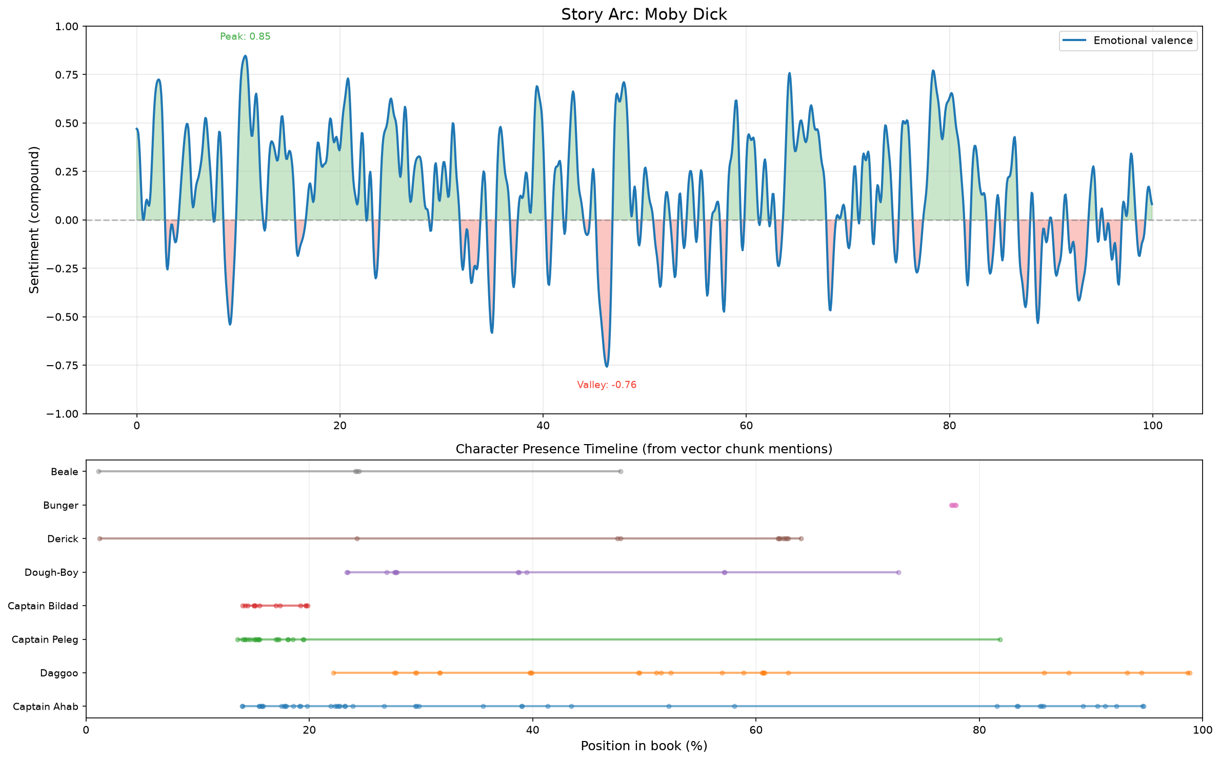
Moby Dick. The arc traces Ishmael's descent from the civilized world into Ahab's monomania, looping through the philosophical digressions before spiraling toward the final catastrophe.
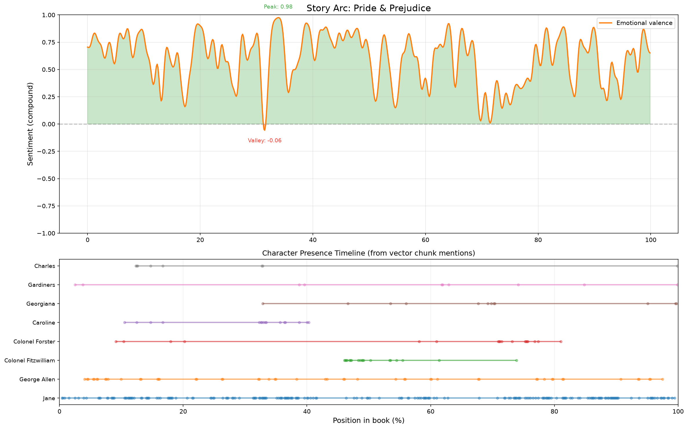
Pride and Prejudice. A tight, symmetrical structure. The arc traces courtship's approach and withdraw pattern, with the emotional center of gravity shifting from Longbourn to Pemberley across the novel.
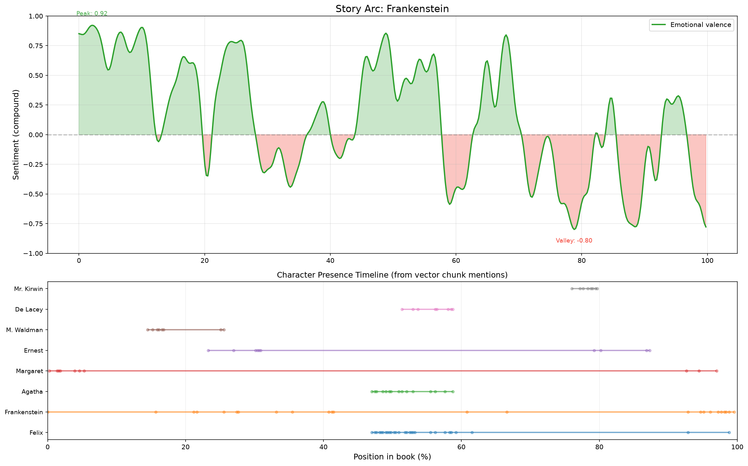
Frankenstein. Three nested arcs for the three narrators (Walton, Victor, the Creature), each orbiting the same central themes of creation and abandonment before collapsing inward.
Act I: Gemma4 and the 350-Word Wall
The Diagnosis
I ran a controlled experiment. Same model. Same book. Same prompt. The only variable was input length.
| Input | Characters extracted | Quality |
|---|---|---|
| 350 words of Moby Dick | 3-9 per passage | ✓ Names correct, verbatim from text |
| 5,700 words of Moby Dick | 0-3 per passage | ✗ Generic descriptors instead of names |
| Full 8,000-token sections × 12 | 0-3 per section | ✗ "The Narrator," "Crew Members" |
The model that extracted "Peter Coffin," "Queequeg," and "Ishmael" perfectly from 350 words of text produced "The Narrator" and "Crew Members" from 5,700 words. This was a sharp cliff, not a gradual degradation. Something in the model's attention mechanism was failing at a specific threshold.
Why 350 Words? The Attention Economics of Structured Extraction
Here is what I believe is happening under the hood. I was not able to confirm this by reading Gemma4's weights , I don't have that kind of access, but the pattern is consistent with the known mechanics of decoder only transformer attention, and it explains the data perfectly.
1. The dual attention constraint.
Structured extraction is not one task. It is two tasks competing for the same attention budget. Task A: attend to the input text to find entity names. Task B: attend to the output schema to generate valid JSON with the correct keys and enum values. In a transformer, every output token is produced by computing attention over all input tokens plus all previously generated output tokens. When the model is generating {"name": "Ishmael", "role": "protagonist"}, it must simultaneously hold the position of "Ishmael" in the input and the schema constraint that "role" must be one of {"protagonist", "antagonist", "supporting"}.
At 500 input tokens, the model computes attention over ~600 positions per output token (500 input + 100 output so far). Each input position gets an average attention weight of 1/500 = 0.002. At 8,000 input tokens, the model computes attention over ~8,100 positions per output token. Each input position gets an average attention weight of 1/8000 = 0.000125. The model has 16 times less attention resolution to pinpoint a specific entity mention in the input.
For a 100 token JSON output, a typical extraction result, the model processes 60,000 attention pairs at 500 input tokens and 810,000 attention pairs at 8,000 input tokens. That is 13.5 times more compute for the same output, with each attention connection carrying 13.5 times less signal.
2. The verbatim copy problem.
To output "Ishmael" as a character name, the model must attend to the exact token position in the input where "Ishmael" appears and copy it verbatim. This is a high precision operation. At 500 input tokens, finding one specific name among 500 positions is a 0.2% precision problem. At 8,000 input tokens, it is a 0.0125% precision problem, sixteen times harder. The model's attention distribution becomes too diffuse to reliably isolate individual entity mentions.
This explains why summarization and question answering still work at long context, those tasks do not require verbatim copying of specific spans. They require semantic understanding, which operates over distributed representations that survive attention dilution. But structured extraction requires pinpointing and copying exact strings from specific positions. That precision does not survive dilution.
3. Residual stream competition.
A transformer's residual stream has finite capacity, in Gemma4's case, 4,096 dimensions across 32 layers. Every piece of information the model needs to track competes for space in this stream. For structured extraction, the model must maintain two competing representations: the input text (with all its entities, relationships, and narrative structure) and the output schema (the JSON structure, the enum values for each field, the formatting constraints).
At 350 words, the input representation is compact enough that the schema state coexists comfortably alongside it. At 8,000 tokens, the input representation expands to fill the available capacity. The schema state gets crowded out. This is exactly what I observed: at long context, Gemma4 stopped following my requested JSON schema and started inventing its own. It returned literary analysis with fields like "summary" and "literary_devices", valid JSON, but not the schema I asked for. The model had lost track of the output constraint because the input had consumed the residual stream budget that was supposed to hold it.
4. The "lost in the middle" effect.
Liu et al. (2023) demonstrated that LLM attention is U shaped, highest at the beginning and end of the context window, lowest in the middle. This is a consequence of how positional embeddings and causal attention interact: tokens at the edges of the context receive disproportionate attention weight because they have fewer neighbors on one side.
At 500 tokens, the "middle" of the context spans roughly positions 100-400. Every position is still within 250 tokens of an edge. The attention trough is shallow, no position is truly lost. At 8,000 tokens, the middle spans positions 1,000-7,000. A character introduced at position 4,000 of an 8,000-token section receives near zero attention weight during generation, regardless of how important they are to the story. The model literally cannot see them. This is a mechanical property of the attention pattern, not a failure of comprehension. The model understands the text. It just cannot attend to position 4,000 while generating output token 47 of a JSON array.
For structured extraction, this means entities in the middle of long sections are systematically invisible. At 350 words, there is no "middle" deep enough to lose entities. At 8,000 tokens, most of the text is in the attention trough.
5. The generation tax.
In a decoder only transformer, every output token generation step recomputes attention over the entire input sequence. This means the cost of generating 100 tokens of JSON grows not with the output length alone, but with the sum of input length and output length. At 500 input tokens, each of the 100 output tokens attends to 600 positions. At 8,000 input tokens, each attends to 8,100 positions. A 16× increase in input produces a 13.5× increase in total attention computation, and a corresponding dilution in per position attention precision for the same model capacity.
For tasks that only need to understand the input (summarization, Q&A), this dilution is manageable because understanding can operate over distributed, coarse grained representations. For tasks that need to copy specific spans from the input (entity extraction), the dilution is fatal because copying requires fine grained, position specific attention.
Taken together, these five mechanisms explain the cliff. It is not that Gemma4 is bad at extraction. It is that structured extraction from long contexts is computationally hostile to models with finite attention budgets. Every model has this cliff somewhere. For Gemma4 on consumer hardware with this prompt complexity, the cliff is at roughly 350-500 words.
The Harness
If the model works at 350 words but fails at 5,000, the answer is not a bigger model. The answer is to never ask the model to annotate more than 500 words at a time.
I built what I call micro extraction: split the book into paragraph aligned windows of roughly 500 words each, extract entity names from each window independently, let KùzuDB's MERGE semantics deduplicate across windows. The model only has to read 500 words and name what it sees, exactly the task it does reliably. The database handles the cross window entity resolution. The window boundaries handle the attention budget.
A full Moby Dick produces about 500 windows. Each window gets one extraction call. Each call stays inside Gemma4's proven effective range.
The trade is more LLM calls for dramatically higher per call accuracy. At $0 marginal cost on local hardware, trading time for quality is the right trade. Moby Dick takes about 2.2 hours. That is slower than the original approach, but the original approach produced four characters, two of them imaginary. Speed without accuracy is not speed, it's waste.
The Speed Problem
The first version of micro extraction was too slow, 4 hours per book. Each window was asking Gemma4 to do too much: character names plus roles plus motivations plus relationships plus themes plus atmosphere, all in one JSON schema. That is six classification tasks bundled into every call. Every additional output field increases the generation tax and consumes residual stream capacity that could be used for input attention.
I split the work into two phases.
Phase 1 asks one thing: "what names do you see?" The output is {"people": ["name"], "places": ["name"], "objects": ["name"]}. No classification. No attributes. No relationships. The model scans, identifies, moves on. Per window time dropped from 20-39 seconds to 7-13 seconds, a 3-5× improvement. The simpler output also stretched the effective input window from 350 words to 500-700 words, because fewer output fields means less schema state competing in the residual stream and less generation tax per window. Fewer windows, each faster.
Phase 2 enriches only the unique entities that Phase 1 discovered. A book with 500 windows and 45 unique characters does 500 cheap name scans and 45 expensive detail calls, not 500 expensive calls. At ~15 seconds per enrichment, Phase 2 adds about 12 minutes. Total per book: ~2.2 hours instead of 4.
The Over Extraction Problem
The name only Phase 1 found everything. Across 30 windows of Moby Dick, roughly the first five chapters, it extracted 50 distinct person names. Four were actual recurring story characters. Eighteen were generic descriptors: "harpooneer," "landlord," "the stranger," "savage," "a white man." Melville withholds Queequeg's name for pages, calling him "the stranger" and "the harpooneer" before revealing it. The model faithfully extracted what the text said, it just was not a name yet. Twenty eight were passing references: "Jonah," "Cato," "Seneca," historical and biblical figures Melville mentions in philosophical digressions and never mentions again.
This was the inverse of the original problem. The detailed v1 prompt under extracted because requiring classification for every entity acted as an implicit filter. When Gemma4 had to assign role: protagonist or character_type: human to "the stranger," it hesitated and omitted the entity entirely. The classification fields were not just slowing things down, they were doing a precision filtering job.
Removing them made the model a scanner instead of a classifier. Scanning finds everything. Classification filters. I had removed the filter without replacing it.
This is a general property of small model structured extraction worth stating explicitly: the more output fields you require, the more conservative the extraction. Classification acts as an implicit precision filter at the cost of recall. Removing it improves recall at the cost of precision. The two concerns, finding entities and describing them, should be separated into different phases, with statistical filtering bridging the gap.
The Frequency Filter
I replaced the implicit classification filter with an explicit statistical one. Real story characters appear across multiple windows. Passing references and generic descriptors appear in one or two and then disappear.
I counted how many windows each name appeared in across Phase 1. Characters appearing in 3 or more windows were kept. Characters appearing in 1-2 were dropped. I also filtered names starting with lowercase letters, common role words (harpooneer, captain, sailor, stranger, landlord), names consisting only of stop words, and names shorter than 3 characters.
This filter runs in pure Python over the Phase 1 results. No LLM call. It removes roughly 92% of the noise from the name extraction pass. The separation of concerns, recall from scanning, precision from statistical filtering, is more reliable than asking the model to do both simultaneously, especially on a model whose attention budget is already strained by the extraction task itself.
Later, I found that the frequency filter should have run between Phase 1 and Phase 2, not after Phase 2. Enriching "harpooneer" and "the stranger" with detailed character profiles wasted GPU time and created nodes that needed cleanup. The lesson: deduplicate and filter before enrichment, not after. The ordering of operations in a pipeline matters as much as the operations themselves.
The Results
I ran the full pipeline overnight on the top 4 books by download count, 6.7 hours on the GTX 1660 Ti. Here is what came out, after post processing:
| Book | Time | Chars | Locs | Rels | Themes |
|---|---|---|---|---|---|
| Moby Dick | 134m | 52 | 136 | 33 | 14 |
| Pride & Prejudice | 84m | 56 | 32 | 100 | 12 |
| Frankenstein | 43m | 22 | 44 | 23 | 12 |
| Hegel | 142m | 106 | 74 | 47 | 14 |
Moby Dick went from 4 characters (2 imaginary) to 52 real characters with 33 typed relationships. The original extraction missed Daggoo, Fedallah, Flask, Cabaco, Perth, Bildad, Captain Peleg, Captain Boomer, and Bunger - actual crew members from the novel. The new extraction found them all. It found actual relationships: Ahab is captain_of Starbuck, enemy of the Parsee, rivalry with Moby Dick. It found themes the original never saw: "fate vs. free will," "man vs. nature," "existential dread," "the sublime."
Pride and Prejudice produced 100 relationships, the most of any book, fitting for a social novel about who is marrying whom. Frankenstein was the cleanest extraction: 22 characters with almost no noise, because the narrative is focused and the cast is tight.
Hegel produced 106 "characters", philosophers mentioned in passing, not story characters. The frequency filter assumes fiction: characters who recur across windows are story significant. In non fiction, the same names recur because the text is about them as historical figures, but they are not characters in a narrative. I have not yet fixed this. The fix would use catalog Subject metadata, "Philosophy", to raise the frequency threshold for non fiction texts.
Post Processing as Engineering
I built a reusable post processing script that applies four fixes across the entire database: name variant merging (305 applied across all books with extraction data), role normalization (635 non canonical roles mapped to the canonical enum), relationship type cleanup, and character type fixes.
The name merging taught me a KùzuDB specific lesson. To merge "Ahab" into "Captain Ahab," I needed to transfer all of Ahab's relationships to Captain Ahab, then delete the Ahab node. Transferring RELATED_TO edges (Character→Character) worked fine - single type relationship tables support MERGE with dynamic endpoints. Transferring INTERACTS_WITH edges did not work at all. INTERACTS_WITH is a multi type relationship table with 11 FROM/TO combinations (Character→Object, Object→Location, Event→Character, etc.). KùzuDB rejects MERGE on multi type tables when endpoint types are ambiguous: "Create rel r2 bound by multiple node labels is not supported."
The fix was to only transfer single type edges explicitly and let multi type edges cascade delete via DETACH DELETE. The lesson is that database schema design choices made during ingestion, like using a single multi type relationship table for cross entity interactions , have downstream consequences for post processing operations that you do not discover until you try to merge nodes.
What the Graphs Look Like
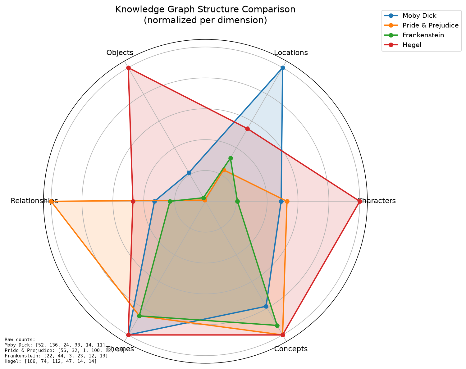
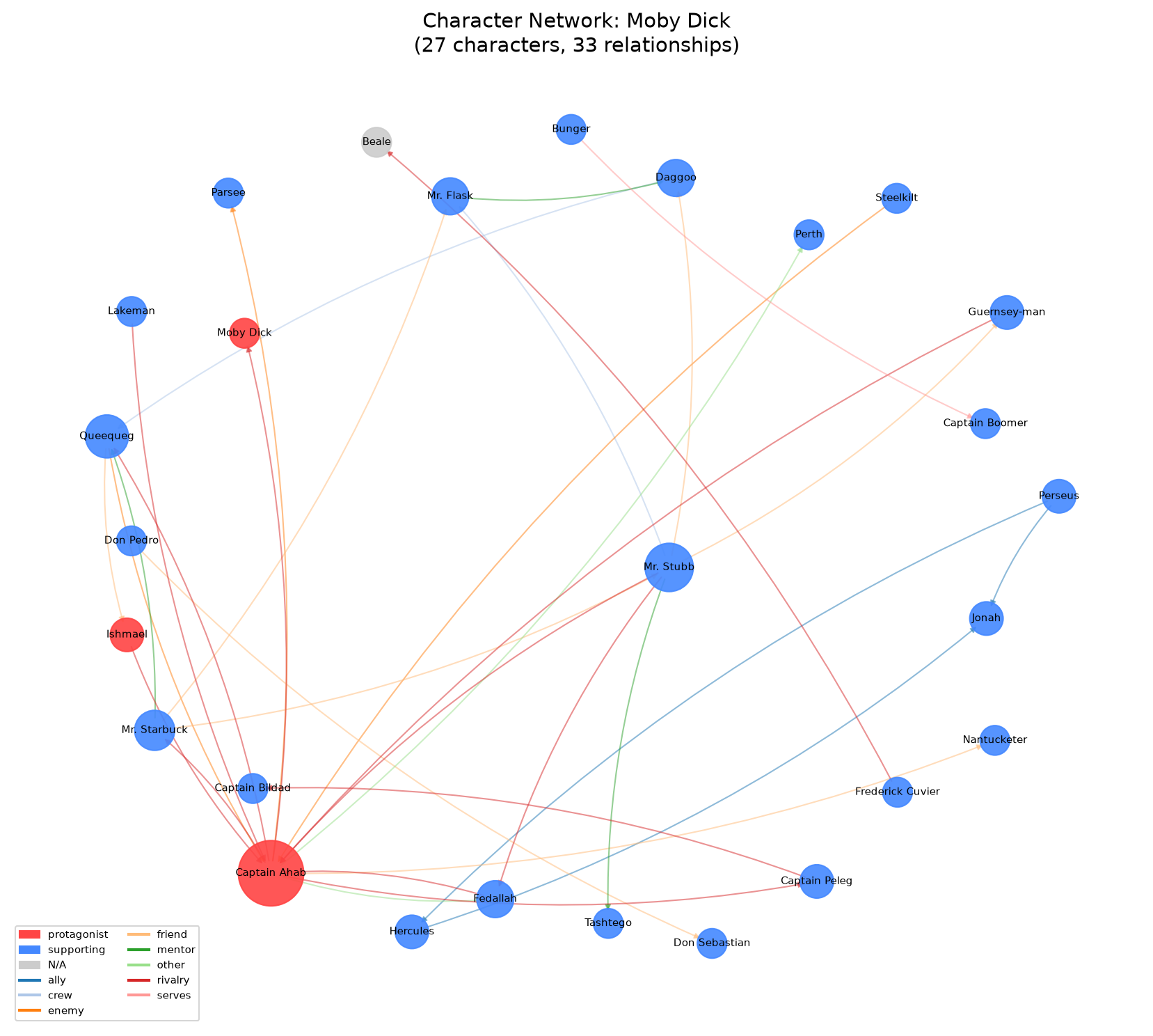
Moby Dick
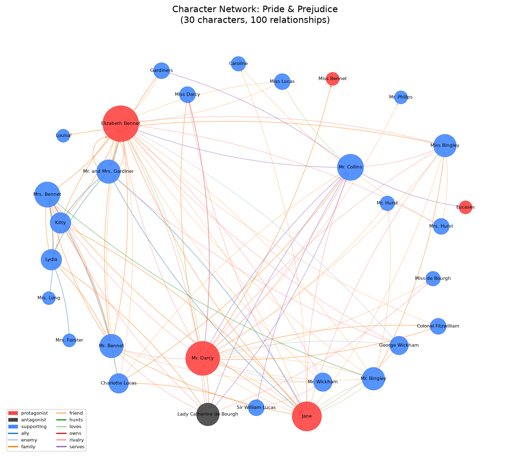
Pride and Prejudice
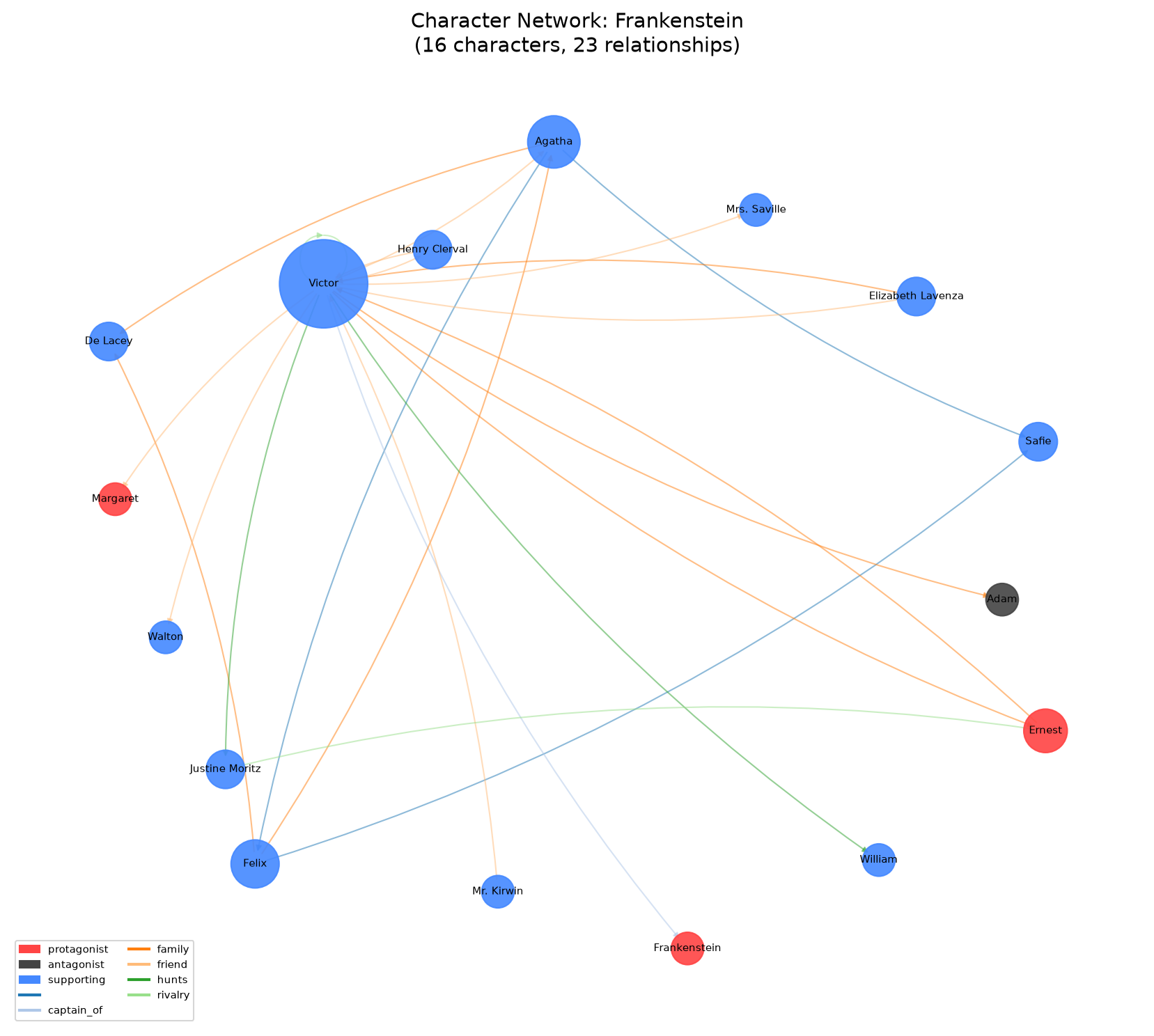
Frankenstein
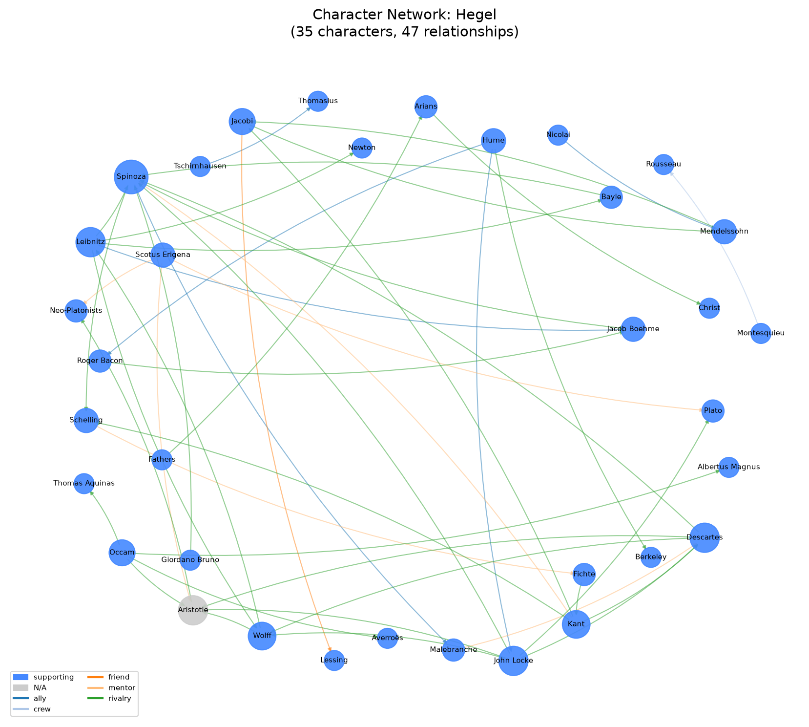
Hegel's Lectures on the History of Philosophy
Act II: LangGraph Learns to Route
How LangGraph Works (The Short Tutorial)
LangGraph models agent systems as directed graphs where nodes are functions and edges are transitions. Here is the anatomy of the graph I built, step by step.
State. Everything flows through a shared state dictionary. I defined mine as a TypedDict:
class GutenState(TypedDict):
    query:          str
    mode:           Literal["auto", "vector", "graph", "hybrid"]
    routed_to:      str
    vector_results: list[dict]
    graph_results:  list[dict]
    cypher:         str
    answer:         str
    messages:       Annotated[list[BaseMessage], add_messages]
The messages field uses LangGraph's add_messages reducer, instead of overwriting the list each time a node returns {"messages": [...]}, new messages are appended. This is the mechanism LangSmith hooks into for tracing: every message added to this list appears as a trace event with the node that produced it.
Nodes. Each node is a pure function (state) → dict. It receives the full state, returns only the fields it wants to update. LangGraph merges the returned dict into the state.
def graph_agent(state: GutenState) -> dict:
    # Generate Cypher via LLM
    cypher = llm.invoke([...]).content
    # Execute against KùzuDB
    rows = conn.execute(cypher)
    # Return updates
    return {
        "graph_results": rows,
        "cypher":        cypher,
        "messages":      [AIMessage(content=f"Returned {len(rows)} rows")],
    }
Graph construction. Nodes are registered with add_node(), edges with add_edge() (unconditional) or add_conditional_edges() (routes based on state). The graph compiles into an immutable executable:
builder = StateGraph(GutenState)
builder.add_node("supervisor",   supervisor)
builder.add_node("vector_agent", vector_agent)
builder.add_node("graph_agent",  graph_agent)
builder.add_node("merge",        merge)

builder.add_edge(START, "supervisor")
builder.add_conditional_edges("supervisor",   _route_supervisor)
builder.add_conditional_edges("vector_agent", _route_vector)
builder.add_edge("graph_agent", "merge")
builder.add_edge("merge", END)

app = builder.compile()  # module-level singleton
Conditional edges. A routing function returns a string literal, the name of the next node. LangGraph enforces that the return type matches the valid targets:
def _route_supervisor(state: GutenState) -> Literal["vector_agent", "graph_agent"]:
    if state["routed_to"] in ("vector", "hybrid"):
        return "vector_agent"
    return "graph_agent"
When user passes mode="vector", the supervisor sets routed_to="vector", and _route_supervisor returns "vector_agent". The conditional edge from vector_agent has its own router: vector goes straight to merge, hybrid continues to graph_agent.
LangSmith integration. Setting LANGCHAIN_TRACING_V2=true is all it takes. LangGraph automatically sends the graph topology, every state transition, and every LLM call to LangSmith. The trace structure mirrors the graph structure, each node execution is a span, each conditional edge decision is logged, and the messages reducer ensures every LLM response appears chronologically in the trace UI.
Making state visible. Here is a lesson I learned the hard way. By default, LangSmith traces show messages but not arbitrary state fields. My graph_results, the actual KùzuDB output, was invisible in traces because it sat in state but not in messages. The fix: have each node append an AIMessage summarizing what it found:
return {
    "graph_results": rows,
    "cypher":        cypher,
    "messages":      [
        cypher_msg,                                    # the generated Cypher
        AIMessage(content=f"Returned {len(rows)} rows  - columns: {col_names}"),
    ],
}
Now the LangSmith trace shows both the generated Cypher AND a summary of what KùzuDB returned, "Returned 20 rows, columns: ['c.name']", directly in the message timeline. No digging through collapsed state panels. The same pattern applies to every node: vector_agent appends "Vector search returned 5 chunks: ['Moby Dick', ...]", merge appends the final answer. Each message becomes a visible trace event.
This is the kind of thing that is obvious in retrospect but easy to miss when you are building: LangSmith shows what you put in messages. If you want to see results, put them there.
The Architecture
With that foundation, here is the query system I built. Four nodes, three conditional edges, compiled at module import time.
The supervisor classifies the user's query as vector, graph, or hybrid. If the user passes an explicit mode flag, it skips classification entirely and uses the flag. This comparison mode is the core of the project: run the same query through vector only, graph only, and hybrid to demonstrate what each backend contributes. The routing is handled by two conditional edge functions that read the routed_to field from state.
The vector agent embeds the query using nomic's asymmetric search_query: prefix, runs ANN search against LanceDB, and returns the top 5 chunks with metadata. The embedding server is a local FastAPI process, a drop in replacement for HuggingFace TEI that I built because TEI's Rust JSON parser rejected nomic-embed-text-v1.5's config.json for having a duplicate field.
The graph agent sends the query plus the full KùzuDB schema plus seven generation rules to the LLM. The LLM returns Cypher. KùzuDB executes it. The merge node synthesizes everything into a final answer.
The Cypher Wars
Gemma4's first attempts at Cypher generation failed in three ways that each taught me something about prompt engineering for small models.
The recency problem. The prompt included the rule "NEVER use exact title match. Always use WHERE b.title CONTAINS 'keyword'" at position 7 in a list. Gemma4 ignored it and used {title: 'Moby Dick'}. I moved the rule to position 1 with explicit WRONG/RIGHT examples, and the model immediately complied. The content of the rule did not change. Its position in the context window did. Small models exhibit stronger recency and primacy effects than large models, rules at the extremes of the prompt are weighted more heavily than rules in the middle. Critical constraints must appear first.
The direction problem. The schema described relationship directions in prose: HAS_ATMOSPHERE FROM Book TO Atmosphere. Gemma4 generated (b)<-[:HAS_ATMOSPHERE]-(a), the arrow pointing the wrong way. I replaced the prose descriptions with explicit Cypher style notation for all eight relationship types: (Book)-[:HAS_ATMOSPHERE]->(Atmosphere). The model immediately generated correct directions. Visual notation communicates directional relationships more reliably than prose because it matches the output format the model is being asked to produce, the model can pattern match the notation directly into the generated query without translating from prose.
The dialect problem. Gemma4 generated FROM, OPTIONAL MATCH, and CALL, Neo4j Cypher features that KùzuDB does not support. KùzuDB implements a subset of openCypher focused on read only graph traversal. I added a rule listing the forbidden keywords and the allowed ones: "NO FROM, NO OPTIONAL MATCH, NO CALL, NO UNWIND. Use only: MATCH, WHERE, RETURN, WITH, ORDER BY, LIMIT, COLLECT, COUNT." The model complied. The lesson is that when a model is trained on Neo4j Cypher examples, it defaults to Neo4j syntax. You must explicitly constrain it to the subset your database supports. The model does not know what database is on the other side of the connection.
After the three fixes, the graph agent produces syntactically valid, directionally correct, KùzuDB compatible Cypher. For the query "what is the atmosphere of Moby Dick and how do the characters contribute to it?", it generates:
MATCH (b:Book) WHERE b.title CONTAINS 'Moby'
MATCH (b)-[:HAS_ATMOSPHERE]->(a:Atmosphere)
MATCH (c:Character)-[:APPEARS_IN]->(b)
RETURN a.name AS Atmosphere, COLLECT(c.name) AS Characters
LIMIT 20
This returns 15 rows, each atmosphere label paired with all 52 characters. Moby Dick's atmosphere is simultaneously "foreboding," "spectral," "meditative," "expansive," "philosophical," and "exhaustion."
The Merge Problem
The hybrid mode's merge node hallucinated. Given 15 graph rows each containing 52 character names, 780 total character references, plus 5 vector chunks of prose, Gemma4 lost track of which book it was analyzing. The answer included "Aunt Polly" from Tom Sawyer, "Captain Nemo" from 20,000 Leagues Under the Sea, and "Peaseblossom" from A Midsummer Night's Dream. None of them are in Moby Dick.
The problem was evidence overflow. The merge prompt plus the evidence block was pushing past Gemma4's effective reasoning range, which is separate from its extraction range but subject to the same attention economics. I applied three fixes:
First, I truncated character lists to 8 per row with "+44 more" notation. The merge LLM does not need all 52 names to understand the pattern, knowing that "a large ensemble of characters contributes to each atmosphere" is sufficient. Truncation is not information loss when the information is redundant.
Second, I added an output format constraint: "Write in prose paragraphs, NOT JSON, NOT markdown tables." Without this, Gemma4 sometimes returned raw JSON arrays, reverting to a format it had seen frequently in training data when uncertain about the task.
Third, I added source grounding: "Only use information present in the evidence. Stay within the book(s) mentioned in the evidence." This is a simple instruction that large models follow implicitly but small models need stated explicitly, the model defaults to drawing on its training data when the evidence is overwhelming, and you have to tell it not to.
After the fixes, the hybrid answer names specific atmosphere labels from the graph and specific characters from Moby Dick, with no cross book contamination.
Act III: LangSmith Shows the Truth
Setup (The Tutorial, Continued)
Three lines of configuration, and LangSmith traces everything:
# .env
LANGCHAIN_TRACING_V2=true
LANGCHAIN_API_KEY=lsv2_pt_...
LANGCHAIN_PROJECT=gutengraph
No code changes. No decorators. LangGraph's SDK detects the environment variables and automatically sends traces. Each node execution becomes a span. Each LLM call within a node becomes a child span. Each state update is logged. The graph topology itself is sent on the first invocation.
For LangGraph Studio, add a langgraph.json at the project root:
{
  "dependencies": ["."],
  "graphs": {
    "gutengraph": "src/gutengraph/agents/graph.py:app"
  },
  "env": ".env"
}
This tells the Studio where to find the compiled graph and how to run it. For local Studio you need Docker (langgraph dev); for cloud Studio, the traces alone populate the graph view at smith.langchain.com.
What the Traces Revealed
Running the atmosphere query through all three modes, LangSmith shows exactly what happens:
The vector only trace: supervisor (LLM classification, ~10s) → vector_agent (embedding + ANN search, ~2s) → merge (evidence synthesis, ~60s). Total: ~75 seconds. The merge node dominates, Gemma4 takes 40-55 seconds to synthesize 700 words of evidence into a coherent answer on a 6 GB GPU. The database queries are sub second. The embedding is sub second. The LLM is the entire latency budget.
The graph only trace: supervisor → graph_agent (LLM Cypher generation, ~15s + KùzuDB execution, <1s) → merge (~60s). Total: ~85 seconds. Cypher generation is fast because the output is short, about 50 tokens. The merge dominates again.
The hybrid trace: supervisor → vector_agent → graph_agent → merge (~70s). Total: ~99 seconds. Both retrieval backends run, the merge receives the largest evidence block, and synthesis takes the longest.
The bottleneck is unambiguous: LLM inference on consumer hardware. A production system would swap Gemma4 for GPT-4o-mini at query time and bring latency from 70-100 seconds to 3-5 seconds, at a cost of roughly $2-5 per month at 500 queries. But for a demo running entirely on a four year old gaming PC, the fact that it works at all is the architecture being validated.
The LanceDB Discovery
One of the vector traces showed an error I had not seen before: "Input/output error (os error 5)." LanceDB was failing to open the vector index. The same LanceDB file worked perfectly when accessed directly from Python, but the LangGraph agent, running in the same Python process, could not open it.
The issue was WSL2’s 9P filesystem protocol. LanceDB is written in Rust and uses mmap for file access. The 9P protocol that WSL uses to mount Windows drives, my LanceDB was stored on /mnt/d, a Windows NTFS drive, does not support the mmap patterns that LanceDB needs. Moving the LanceDB directory to the native ext4 filesystem at /home/hijaz/projects/gutengraph/data/lancedb fixed the issue permanently.
Without LangSmith’s trace, I would have seen “sometimes the query fails” and spent hours trying to reproduce it. With the trace, I could see exactly which node failed, with what error, on which file access. The trace pointed directly at the cause. This is the difference between debugging with observability and debugging with print statements.
What LangGraph Studio Showed
A langgraph.json config file connects the project to LangSmith’s cloud Studio. The graph topology is visualized as a directed graph with conditional edges highlighted. I could see the supervisor branching to vector_agent or graph_agent based on the classification result. I could see the vector_agent conditionally routing to merge or graph_agent based on whether the mode was hybrid. I could step through node executions, inspect state at each transition, and replay runs with modified inputs.
For a system where the routing logic is the core intellectual property, where the comparison between backends is the thesis, being able to visually verify that the routing is correct for every mode is essential. One conditional edge pointing the wrong way would silently corrupt every hybrid query. Studio makes that impossible to miss.
Epilogue:Nine Things I Now Know
1. Model cards lie about context windows.
A model’s advertised context length is for reading. Its effective context for structured annotation is an order of magnitude smaller. The difference is the dual attention constraint: reading only requires understanding, but annotation requires understanding plus verbatim copying plus schema adherence, all competing for the same attention budget. Every model has this cliff somewhere. Find it by testing, not by reading the spec sheet.
2. The harness does not improve the model. It designs around the model’s limits.
Micro extraction does not make Gemma4 better at extraction. It makes the task fit inside the attention budget where Gemma4 already works. The database handles deduplication. The windows handle input sizing. The frequency filter handles precision. The model only has to read 500 words and name what it sees, the one thing it does reliably.
3. Output schema complexity determines effective input length.
The more fields you ask for, the shorter the input the model can handle before structured extraction degrades. The classification fields in the detailed prompt were consuming residual stream capacity and generation budget that could have been used for input attention. Removing them stretched the effective window from 350 to 500 words. The relationship is causal: simplify the output, and the usable input expands.
4. Classification is an implicit filter with a predictable cost.
Requiring the model to classify every entity it extracts raises precision at the cost of recall. Removing classification requirements raises recall at the cost of precision. These concerns should be separated: let the model scan (high recall, cheap), then filter in post processing (high precision, even cheaper). Do not ask a model with finite attention to do both simultaneously.
5. Prompt ordering matters as much as prompt content.
A rule at position 7 in a prompt got ignored. The same rule at position 1 got followed exactly. The content did not change, the position in the context window did. Small models exhibit stronger serial position effects than large models. Critical constraints must appear first. Examples with explicit WRONG/RIGHT pairs communicate better than prose instructions. Visual notation - (Book)-[:HAS_ATMOSPHERE]->(Atmosphere), communicates directional relationships more reliably than declarative descriptions.
6. LangSmith shows what you put in messages, not state.
LangSmith traces display the messages list beautifully. Arbitrary state fields like graph_results or vector_results are technically logged but buried in collapsed JSON panels that nobody checks. The fix is straightforward: have every node append an AIMessage summarizing its output. “Cypher returned 20 rows” or “Vector search returned 5 chunks: [‘Moby Dick’, ‘Dracula’]” , these show up directly in the trace timeline as visible events. If you want to see it in LangSmith, put it in messages.
7. Observability is infrastructure, not a feature.
LangSmith traces turned a "sometimes it fails" bug into a "here is exactly which filesystem call failed" diagnosis. The LanceDB WSL issue would have been hours of guesswork without it. LangGraph Studio turned a "did the routing work?" question into a visual inspection. For multi agent systems where correctness depends on conditional edges firing correctly, visual verification of the graph topology is not optional.
8. The dual brain architecture works, within constraints.
Vector search gives atmosphere and texture. Graph traversal gives structure and enumeration. The hybrid mode combines them, but only when the evidence fits inside the merge model's effective reasoning range. The three mode comparison, same query, three different retrieval paths, demonstrates exactly what each backend contributes. That comparison is the thesis of the project, and it holds up under scrutiny.
9. Rule based sentiment tools break on irony.
VADER, the lexicon based sentiment analyser I used to trace the story arcs, completely failed on Jane Austen. Her surface vocabulary is so relentlessly genteel that a rule based system reads every scene as positive, missing the irony that is the entire point. The Pride and Prejudice arc came out absurdly cheerful because "I am excessively diverted" registers as joy when it is, in context, a razor. Embedding based analysis catches what lexicon based tools miss because embeddings encode contextual usage, not dictionary definitions. When your tool relies on word lists, it will fail on any writer whose art is the gap between what words mean and what they do.
All code, test scripts, raw extraction results, and the full engineering log are in the GütenGraph repository. Everything described here is reproducible with any 6-8 GB consumer GPU running Ollama + gemma4.