LLM Internals: The Crozzled Heart

GPT-2 is 124 million parameters. That is 496 megabytes of floating point numbers in a folder on my laptop. I can pick it up and hold it on a USB stick. I can load it onto a GPU from 2019 and watch it generate text that is, occasionally, indistinguishable from something a person might write.

Somewhere inside those 496 megabytes, a single file small enough to fit comfortably in the RAM of a phone, is a compressed representation of everything GPT-2 knows. It knows the capital of France. It knows that if you drop a ball, it falls. It knows the plot of Hamlet, approximately. It knows how to write a resignation letter, a wedding toast, a limerick about a man from Nantucket. All of it, ten thousand dreams, is ensepulchred within matrix multiplications and layer normalizations.

Mechanistic interpretability is the attempt to open it. Not to explain what a model can do, benchmarks do that, but to explain how it does it. To find the specific circuits, attention heads, and neurons that implement specific behaviors. To go from “this model can conjugate verbs” to “this attention head at layer 5 attends to the token that carries tense information, and this MLP neuron at layer 7 boosts the logit for the correct suffix, and here is the weight matrix that connects them.”

Chapter 1: A Cold Light

We type a prompt into the box, wait for the box to glow, and read the text that comes out. If the box says something wrong, we tweak the prompt and try again.

This is the “It Just Works” Illusion. It judges the model purely by its behavior.

Mechanistic interpretability rejects this. We do not want to just know what the model does; we want to know how it does it. We want to reverse engineer the compiled weights back into readable source code. If a model knows that the capital of France is Paris, we want to find the exact circuit that looks up “France,” the wire that transmits “capital,” and the gears that output “Paris.”

Before we can perform brain surgery on a neural network, we need to understand how it reads data, and we need to set up our operating table.

Tokens to Vectors: The On Ramp

Neural networks cannot read English. They cannot read punctuation. They only understand numbers of a fixed size. To get our text into the model, it has to go through a two step translation process.

1. Tokenization

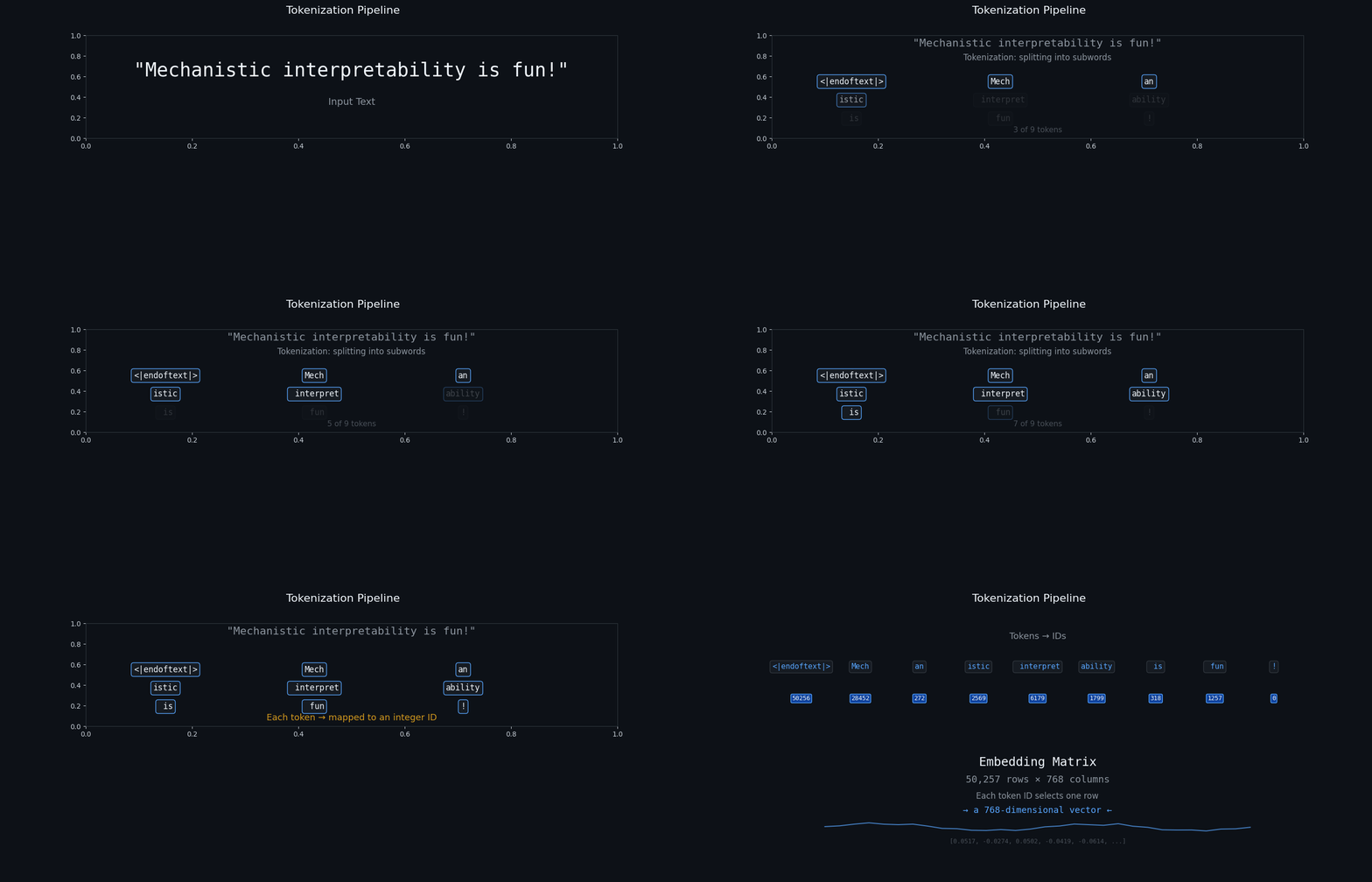
The model does not read word by word or character by character. It reads in chunks called tokens. A token can be a whole word, a syllable, or just a single letter.

“Apple” might be one token.

“Mechanistic” might be three tokens: “Mech” + “an” + “istic”.

Every token is mapped to a specific integer ID in the model's vocabulary. If GPT-2 has a vocabulary of 50,257 tokens, then our prompt is just a list of integers between 0 and 50,256.

2. The Embedding Matrix

Integers are not enough. Token IDs are arbitrary labels. The token with ID 4,000 is not “twice” the token with ID 2,000; the numbers are just slots in a vocabulary, assigned during training, with no arithmetic meaning. But a neural network does nothing but arithmetic. Feed it the raw ID 4,000 and it will happily treat that number as twice as large as 2,000, which is nonsense. So the model uses an Embedding Matrix, a massive lookup table that converts each arbitrary ID into a vector the network can actually compute with.

For GPT-2 Small, this matrix has 50,257 rows, one for every token, and 768 columns. That 768 is the model's embedding dimension, the width of the residual stream we will follow through the entire network in the next chapter; every token, every layer, every internal computation lives in this same 768 dimensional space. When we feed the model the token ID for “cat”, it goes to the “cat” row and pulls out a list of 768 floating point numbers.

This 768 dimensional vector is the mathematical representation of the token. It is what actually enters the model's neural network.

Here is what happens when we run this:

import torch
from transformer_lens import HookedTransformer

# Turn off gradients to save memory, we are dissecting, not training
torch.set_grad_enabled(False)

print("Loading GPT-2 Small...")
model = HookedTransformer.from_pretrained("gpt2-small")
print("Model loaded successfully!\n")

prompt = "Mechanistic interpretability is fun!"

# Convert string to token IDs
tokens = model.to_tokens(prompt)
print(f"Token IDs:\n{tokens}\n")

# Convert IDs back to string chunks to see the exact splits
str_tokens = model.to_str_tokens(prompt)
print(f"String Tokens:\n{str_tokens}")

And here is the output:

Loading GPT-2 Small...
Model loaded successfully!

Token IDs:
tensor([[50256, 28452,   272,  2569,  6179,  1799,   318,  1257,     0]])

String Tokens:
['<|endoftext|>', 'Mech', 'an', 'istic', ' interpret', 'ability', ' is', ' fun', '!']

Several things to notice here. First, TransformerLens prepends a <|endoftext|> token (ID 50256) by default (prepend_bos=True). In GPT-2's training, this token was a document separator between web pages; TransformerLens reuses it as a start of sequence marker.

Second, look at how “Mechanistic” is split: “Mech” (28452), “an” (272), “istic” (2569). Three tokens. This is Byte Pair Encoding in action, a compression algorithm that finds the most common subword chunks in the training data. The model has never seen “mechanistic” as one word. It has seen “Mech” in mechanical, mechanic, mechatronics; “an” in a million places; and “istic” in characteristic, artistic, futuristic.

Third, notice the spaces: “ interpret” and “ is” and “ fun” carry leading spaces, but “ability” does not. In GPT-2's vocabulary, spaces are part of the token, not separate characters. A token starting with a space means “this token begins a new word.” A token without a leading space means “this token continues the previous word.” “ interpret” starts the word, and “ability” continues it: together they form “interpretability.”

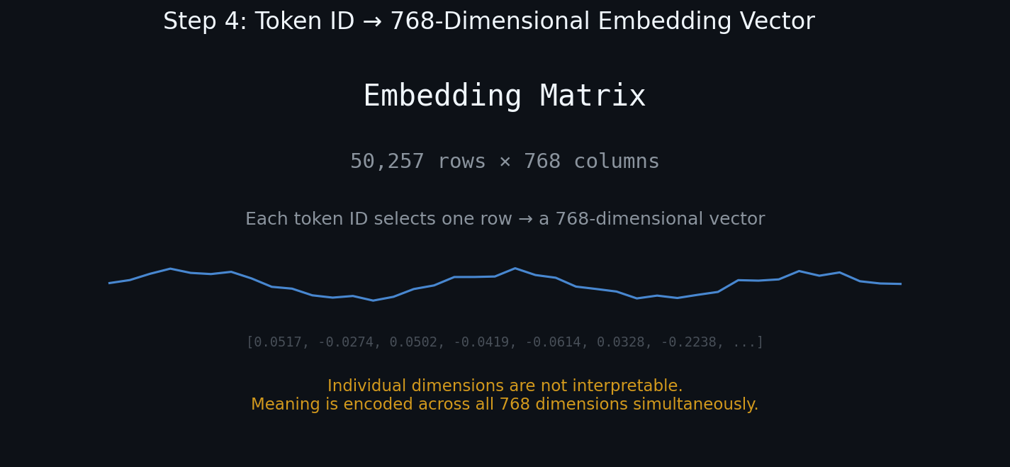
The embedding matrix that these IDs look up has shape [50257, 768]. 50,257 rows, the vocabulary plus the end of text token, 768 columns. When we look up token 50256, we get a vector of 768 numbers. The first eight are:

[0.0517, -0.0274, 0.0502, -0.0419, -0.0614, 0.0328, -0.2238, -0.0871]

These numbers are not interpretable individually. A single dimension in an embedding vector does not correspond to a human concept like “noun” or “color” or “positive sentiment.” It participates in a distributed representation: meaning is encoded across all 768 dimensions simultaneously, in the pattern of interactions between them. The vector for “king” is close to the vector for “queen” in embedding space, and the vector for “king” minus “man” plus “woman” lands near “queen,” but the individual dimensions of any one vector are just noise.

This is why “king minus man plus woman lands near queen” works at all. If each word owned a neuron, that subtraction would be gibberish, you cannot subtract one cell from another. It works because “royalty,” “maleness,” and “femaleness” are directions in the space, arrows you can add and subtract. There is no row labeled “king” to look up; there is only how strongly the vector points along each arrow. Slide along the gender arrow, keep the royalty arrow, and you arrive at queen. Knowledge you can do arithmetic on is knowledge stored in directions, not places.

This is the first lesson of mechanistic interpretability: the model's knowledge is not stored in places. It is stored in directions.

Chapter 2: The Spine

We have GPT-2 Small loaded. We type a prompt. A moment later, text comes out. But what happens in the milliseconds in between?

To understand a neural network, we cannot just look at the input and the output. We have to look at the main artery connecting them. In transformer models, this artery is called the residual stream.

The Main Highway

Think of the residual stream as a high bandwidth pipe. It starts at the embedding layer and runs straight through to the very end of the model.

The most important mathematical rule of the residual stream is simple addition. As our token vector travels down the stream, it encounters Layer 0. Layer 0 does not intercept and replace the vector. Instead, it reads from the stream, does some calculations, and adds its results back in.

The updated vector then moves to Layer 1, which reads the new state, calculates, and adds its own updates. This happens 12 times in GPT-2 Small. The stream is the model's working memory, accumulating context and meaning at every step. Nothing is ever overwritten. Everything is accumulated.

The X-Ray Machine: The Logit Lens

If the residual stream is just an evolving list of 768 numbers, how do we know what the model is thinking at Layer 6?

At the very end of the model, there is an Unembedding Matrix. Its job is to take the final, highly processed 768 dimensional vector and project it back into the model's vocabulary to predict the next word.

But we do not have to wait until the end.

Because the residual stream uses addition, the data format remains exactly the same at every layer. The vector at Layer 4 has the same shape as the vector at Layer 11. We can take the vector from any layer, skip the rest of the network, and multiply it directly against the Unembedding Matrix.

By applying this projection at every layer, we can watch the model's internal guess sharpen in real time. This is the Logit Lens.

Here is the code:

import torch
from transformer_lens import HookedTransformer

torch.set_grad_enabled(False)
model = HookedTransformer.from_pretrained("gpt2-small")

prompt = "The Eiffel Tower is located in the city of"

# run_with_cache intercepts the residual stream at every layer automatically
logits, cache = model.run_with_cache(prompt)

And here is what the model thinks at every layer:

=== Logit Lens: Top prediction after each layer ===
  Layer  0:  top-5: [' the', ' course', ' a', ' our', ' its']
  Layer  1:  top-5: [' the', ' course', ' its', ' our', ' late']
  Layer  2:  top-5: [' course', ' the', ' late', ' Hum', ' its']
  Layer  3:  top-5: [' course', ' the', ' Gran', ' Gat', ' Towns']
  Layer  4:  top-5: [' La', ' Towns', ' Gran', ' course', ' Bern']
  Layer  5:  top-5: [' England', ' La', ' Gat', ' Indianapolis', ' Wisconsin']
  Layer  6:  top-5: [' Naples', ' southwest', ' Georgia', ' Ing', ' England']
  Layer  7:  top-5: [' Ing', ' Naples', ' Gat', ' Rome', ' Chicago']
  Layer  8:  top-5: [' Rome', ' Chicago', ' Ing', ' London', ' Houston']
  Layer  9:  top-5: [' Amsterdam', ' London', ' Paris', ' Hamburg', ' Cologne']
  Layer 10:  top-5: [' Amsterdam', ' Hamburg', ' Berlin', ' Paris', ' Cologne']
  Layer 11:  top-5: [' Amsterdam', ' Hamburg', ' Paris', ' Cologne', ' Berlin']

  Final:  top-5: [' London', ' Paris', ' Amsterdam', ' Berlin', ' New']

A few things to notice.

The model does not converge monotonically. It does not start fuzzy and gradually sharpen toward the right answer. It lurches. At Layer 0, it is 70% confident the next word is “the”, a generic, grammatically safe guess. By Layer 3, it has abandoned “the” for place names: “Gran,” “Gat,” “Towns.” It knows a location is coming. At Layer 5, it commits to “England” at 81%, wrong level of specificity, right domain. At Layer 7, something bizarre happens: “Ing” spikes to 99.8%. I still do not have a clean explanation for this. It looks like the model is trying to complete a word fragment, perhaps an intermediate representation of a city name like “Inglewood” or some grammatical computation bleeding into the vocabulary projection. Then Layer 9 commits to “Amsterdam” at 98.7%, and Layers 10 and 11 harden that to near 100%.

And then the final output gives us: London (29%), Paris (28.9%), Amsterdam (16.9%), Berlin (13.5%). The final distribution is flatter than the intermediate ones. The model spent three layers certain about Amsterdam, then walked it back.

Paris is never the top prediction at any intermediate layer. It appears at rank 3 in Layer 9, rank 4 in Layer 10, rank 3 in Layer 11. The correct answer is present, but it is never dominant. The model is not “thinking Paris” and then saying Paris. It is thinking Amsterdam, Amsterdam, Amsterdam, and then, at the very last step, distributing probability across London, Paris, Amsterdam, and Berlin.

Layer 5's “England” is a country, not a city. The model knows the prompt is asking for a location, but it has not resolved the granularity yet. It grabs the concept of “place in Europe” and the nearest token is “England.” This is concept retrieval, not prediction. The model has activated the England region of its representation space, but that region contains cities, countries, landmarks, and languages. The unembedding matrix picks the closest token it can find, which is “England,” close, but wrong granularity.

When the Microscope Lies: The Logit Lens Illusion

The Logit Lens is powerful, but it can trick us.

When we project a middle layer's vector into the vocabulary and see “Amsterdam” at 98.7% probability, we might assume the model is actively predicting “Amsterdam” as the next word. Not necessarily.

The model might just be gathering the concept of “European capital city where they speak a language other than English” to use later in a calculation, perhaps to narrow the set of possible completions, or to activate the right grammatical frame for a location preposition. The unembedding matrix is greedy. It will translate any European capital adjacent data in the stream into the closest matching vocabulary token, which at Layer 9 happens to be “Amsterdam.”

Look at the final output again: “London” at 29%. London. The capital of England. Layer 5 activated “England.” The model was not predicting England as the answer. It was retrieving the concept in order to reason toward London. But if we had only looked at Layer 5 through the Logit Lens, we would have drawn the wrong conclusion.

Always ask: is the layer predicting this word, or just gathering concepts related to it?

There is a second illusion, quieter than the first. The numbers themselves are sensitive to how you read them. A logit lens that projects the raw residual stream straight to the vocabulary, as mine does, looks noticeably more erratic than one that applies the model's final layer normalization first, the same ln_final the real unembedding sees. Had I applied it, the Layer 7 “Ing” spike and the three layers certain about Amsterdam would be less dramatic, though still present. The intermediate layers were never trained to be read either way, so some of the lurching is the model thinking and some is the lens straining to translate a vector that was never meant to be projected yet. The Logit Lens does not have a calibrated zero. Treat the trajectory as a story about direction, not a transcript of confidence.

The residual stream is not a narrowing funnel toward the right answer. It is a scratchpad where the model writes, rewrites, and sometimes erases. The Logit Lens shows us the scratchpad at each step. But reading the scratchpad correctly requires understanding that not everything written on it is a prediction. Some of it is just thinking.

Chapter 3: The Watchers

The residual stream carries context forward, but it does not do any thinking on its own. The actual computation happens in the layers that read from the stream. The first major computational engine we encounter is the attention mechanism.

If the residual stream is a highway, attention heads are the scouts. They look back at previous tokens, figure out which ones are relevant to the current token, and move information between them.

Who Is Looking at Whom: The Two Circuits

A single attention head is made of two separate, smaller circuits working together. We break them down into the QK Circuit (Query Key) and the OV Circuit (Output Value).

1. The QK Circuit: The Matchmaker

Imagine every token at a networking event.

The Key vector is a token's nametag. It broadcasts: “Here is who I am and what context I hold.”

The Query vector is a token's clipboard. It broadcasts: “Here is the specific information I am looking for.”

When the model processes a prompt, the QK circuit calculates the dot product between every token's Query and every previous token's Key. If the dot product is high, the match is strong. The current token will pay attention to that past token. The result of all these match scores is a grid called the Attention Pattern.

2. The OV Circuit: The Delivery System

Once a match is made, information has to be transferred.

The Value vector contains the actual data the past token wants to send. The Output matrix takes that data and reshapes it so it fits back into the 768 dimensional residual stream.

In short: QK decides where to move information. OV decides what information to move.

Induction Heads: Learning to Copy and Paste

Before the experiment, two pieces of vocabulary that the rest of this chapter leans on: the current token and the previous tokens.

The current token is the one the model is processing right now, the position it is about to predict from. In a prompt, that is always the last token. The previous tokens are everything to its left. Attention is causal: a token may look back at itself and everything before it, but never forward. So the current token is where the model is standing, and the previous tokens are its entire view to the left.

With that fixed, the Induction Head is easy to describe. It is one of the most famous discoveries in mechanistic interpretability, a specialized attention head that develops naturally as language models get larger, and its entire job is to copy and paste repeating text.

Suppose we feed the model: “Mr. Smith went to the store. Then Mr.” The current token is the final “Mr.” An induction head runs a specific algorithm on it: take the current token, look back through the previous tokens for the last place that same token appeared, shift forward by exactly one position, and copy whatever followed it. The earlier “Mr.” was followed by “Smith,” so the head grabs “Smith” through its OV circuit and writes it into the current residual stream, all but guaranteeing the model predicts “Smith” next. The rule in one line: attend to whatever followed the last time the current token appeared.

That is the clean story. The real weights are messier, and seeing exactly where they diverge is the point.

Here is the experiment:

import torch
from transformer_lens import HookedTransformer

torch.set_grad_enabled(False)
model = HookedTransformer.from_pretrained("gpt2-small")

# A prompt with a clear repeating pattern
prompt = "Mr. Dursley was a beefy man. Mr."

logits, cache = model.run_with_cache(prompt)

# Attention pattern from Layer 5
# Shape: [batch, head_index, query_position, key_position]
attention_pattern = cache["blocks.5.attn.hook_pattern"]

# Isolate Head 5 for the first batch item
head_5_pattern = attention_pattern[0, 5, :, :]

# Attention FROM the final token (the period after "Mr.") looking backward
last_token_attention = head_5_pattern[-1, :]
tokens = model.to_str_tokens(prompt)

print("Attention from the final '.' token looking backward:")
for token, score in zip(tokens, last_token_attention):
    print(f"  {token:12} : {score.item() * 100:.2f}%")

And here is the output:

Before reading the numbers, look at how the prompt actually tokenizes, because the current token is not the one you would guess:

0:  <|endoftext|>   (BOS, prepended by TransformerLens)
1:   Mr
2:  .
3:   D
4:  urs
5:  ley
6:   was
7:   a
8:   beef
9:  y
10:  man
11: .
12:  Mr
13: .

“Mr.” is not a single token. It splits into “ Mr” and “.”, so the last token in the prompt, the current token, is the period at position 13, not “Mr.” This is why the code reads head_5_pattern[-1, :]: the -1 selects the final position, the period. Everything in the output below is that period looking backward over positions 0 through 12, its previous tokens.

Attention from the final '.' token looking backward:
  <|endoftext|> : 77.88%
  Mr            :  0.39%
  .             :  0.42%
   D            : 14.97%
  urs           :  0.01%
  ley           :  0.02%
   was          :  0.20%
   a            :  0.47%
   beef         :  1.28%
  y             :  0.01%
   man          :  0.60%
  .             :  1.52%
   Mr           :  1.82%
  .             :  0.42%

Several things to notice.

The BOS sink. <|endoftext|> gets 78% of the attention. This is the model's null position. When a head has no strong opinion about where to attend, it dumps its attention budget into the first token. Almost every head in GPT-2 does this. It is the attentional equivalent of “I do not know.” In the full attention matrix, every single token from position 0 through 13 gives the BOS token at least 59% of its attention. This head is only occasionally doing its actual job.

The induction signal. The second strongest signal is “ D” at 15%, and this is induction firing. The current token, the period at position 13, is preceded by “ Mr”. It looks back through the previous tokens for an earlier period in the same situation, one also preceded by “Mr”. There are two earlier periods to choose from: position 2 (preceded by “Mr”) and position 11 (preceded by “man”). Only position 2 matches. The head locks onto it, shifts forward by exactly one token, and lands on “ D” at position 3, the start of “Dursley.” Attend to whatever followed the last time the current token appeared. The head is doing induction. It is just doing it quietly, underneath a mountain of BOS attention.

The model still gets it right. Despite the messy attention pattern, the model's final prediction is:

Final top-5 predictions: [' D', ' Mc', ' M', ' G', ' B']
Probabilities: ['0.966', '0.009', '0.009', '0.008', '0.008']

“ D” at 96.6%. That is Dursley's initial. The model saw the pattern of a period following “Mr” and knew a surname beginning with D was coming next. The induction mechanism worked. It just took a distributed effort across multiple heads and layers, not a single clean circuit in Head 5 of Layer 5.

This is the reality of mechanistic interpretability. The diagrams in papers show clean, single purpose circuits. The actual weights show heads that are 78% doing nothing, 15% doing their advertised job, and the rest split across noise. The behavior emerges from the aggregate.

What We Actually Found

The full attention matrix confirms the picture. Here is every token's attention distribution in Head 5, Layer 5:

            <|endoftext|>      Mr       .       D     urs     ley     was ...
<|endoftext|>  100.0     .      .      .      .      .      .
          Mr   99.7     .      .      .      .      .      .
           .   99.4     .      .      .      .      .      .
           D   99.8     .      .      .      .      .      .
         ...   (nearly every token gives >90% to BOS)
           Mr   59.0     .    14.8   16.6     .      .      .
           .    77.9     .      .    15.0     .      .      .

The last two rows are the only interesting ones. The second “Mr.” (59% BOS) splits its remaining attention between the period after the first “Mr.” (14.8%) and the “ D” that begins “Dursley” (16.6%). The model is tracing the pattern: find the previous “Mr.”, look at what came after it, and use that to predict what comes next.

The general lesson: attention heads in small models are rarely specialists. They are generalists with a preference. Head 5 at Layer 5 prefers induction, but it spends most of its time staring at the BOS token. The clean circuit diagrams in papers are the result of careful isolation, not a photograph of what any single head is doing at any single moment.

Chapter 4: The Reliquary

Attention heads are fantastic at moving information around. If we ask a model to summarize a document, the attention heads do the heavy lifting by copying words from earlier in the text.

But what if we ask the model a trivia question? If we prompt it with “The capital of France is,” the word “Paris” is nowhere in the text. The attention heads cannot copy it. The model has to pull that knowledge from deep inside its own brain.

That knowledge lives in the Multi-Layer Perceptron (MLP) layers, and to see why it has to, we need to be clear about the order of events inside the model. Attention and the MLP are not two phases that run once each. Every one of the 12 blocks contains both: attention first, then an MLP, and the next block does the same, twelve times over. The two halves divide the labor cleanly. Attention moves information sideways, between token positions; it is the only thing in the model that lets one position see another. The MLP works straight up, within a single position; it never looks at other tokens, it only reads whatever is sitting in the residual stream at its own position and adds to it.

That second fact is the key to fact retrieval. Because the MLP is position local, the ingredients of a question have to already be present at a position before the MLP there can answer it, and the only thing that can deliver them is attention. With “The capital of France is,” attention at the last position spends the early layers reaching back and pulling “France” and “capital” forward into that position's stream. Once those concepts are co located, an MLP can read “France + capital” locally and inject “Paris,” which is nowhere in the text to be copied. This is why the chapter's whole premise holds: the attention heads cannot retrieve the fact, they can only assemble the query; the MLP supplies the answer from its stored weights. If attention heads are the scouts routing information, the MLP layers are the massive filing cabinets where the model stores its factual knowledge.

The Key Value Memory View

To understand how an MLP stores facts, we have to look at its two distinct halves. Researchers like Mor Geva discovered that we can treat these two halves like a giant key value database.

1. The Key Matrix (W_in)

The first half of the MLP reads from the residual stream. It acts as a set of pattern matchers. You can think of each neuron in this layer as a “key” waiting for a very specific signal.

One neuron might be tuned to activate only when it sees the concept of “France” mixed with the concept of “capital cities.”

2. The Activation Function (The Gatekeeper)

Once the Key matrix calculates its matches, the results pass through an activation function (GELU, in GPT-2's case). This acts as a strict threshold. If the match is weak, the activation function sets the value close to zero. The neuron stays quiet. If the match is strong, the neuron fires.

3. The Value Matrix (W_out)

When a neuron fires, it triggers the second half of the MLP. This matrix holds the “values.” If our “France + capital” neuron fires, the Value matrix is wired to output the mathematical concept of “Paris” and add it directly into the residual stream.

The residual stream moves forward, now enriched with the knowledge that the answer is Paris.

Calling this a database is a useful lie. There are no addresses and no exact keys. A query does not look up a row; it partially matches every key at once, and the strongest matches release their values into the stream. It is content addressable by direction, not by location, which is the same lesson from Chapter 1 wearing a different coat.

The Expansion Workspace

The residual stream in GPT-2 Small is exactly 768 dimensions wide. It never changes size.

However, the model knows a lot of facts. Trying to evaluate all those facts in a cramped 768 dimensional space is impossible. To fix this, the MLP does something clever: it expands.

The Key matrix projects the 768 dimensional vector up into a massive 3,072 dimensional workspace. This gives the model thousands of independent neurons to check for thousands of different concepts simultaneously. After the neurons fire, the Value matrix compresses the result back down to 768 dimensions so it can slide back onto the residual stream highway.

Opening the Vault

Let us look inside. We feed the model a simple sentence and inspect the MLP activations at Layer 8:

import torch
from transformer_lens import HookedTransformer

torch.set_grad_enabled(False)
model = HookedTransformer.from_pretrained("gpt2-small")

prompt = "I took a flight to Paris, France."

logits, cache = model.run_with_cache(prompt)

# MLP activations in Layer 8, after the activation function fires
# Shape: [batch, position, d_mlp] -> [1, 10, 3072]
mlp_activations = cache["blocks.8.mlp.hook_post"][0]

# Count how many neurons fired per token
for i, token in enumerate(model.to_str_tokens(prompt)):
    n_active = (mlp_activations[i, :] > 0).sum().item()
    pct = n_active / 3072 * 100
    print(f"  {token:16} : {n_active:4d} active ({pct:5.1f}%)")

And here is the output:

  <|endoftext|>    :  767 active ( 25.0%)
  I                :  403 active ( 13.1%)
   took            :  472 active ( 15.4%)
   a               :  536 active ( 17.4%)
   flight          :  378 active ( 12.3%)
   to              :  527 active ( 17.2%)
   Paris           :  269 active (  8.8%)
  ,                :  421 active ( 13.7%)
   France          :  285 active (  9.3%)
  .                :  450 active ( 14.6%)

A few things worth noting.

The MLP is sparse. At most, 25% of the 3,072 neurons fire for any given token. For content tokens like “Paris” and “France,” the number drops to 8.8% and 9.3% respectively. Over 90% of the neurons in the expanded workspace are silent at any moment. This is the gatekeeper at work: the activation function zeros out anything below threshold, and most concepts are not relevant to any single token.

The BOS token activates the most neurons. 767 neurons (25%) fire for <|endoftext|>. This is the model's idle state. When there is no content to process, the MLP is still doing something: maintaining a default representation, priming itself for the tokens to come.

“Paris” and “France” have the fewest activations. Only 269 and 285 neurons respectively. This seems counterintuitive: should not a fact lookup trigger MORE neurons? But it is the opposite. The more specific the concept, the more targeted the activation. A generic token like “a” fires 536 neurons because it needs to be ready for many possible continuations. “Paris” fires 269 because it knows exactly what it is.

The Neuron That Would Not Stop

There is something else in the data. Let us look at which neuron fires hardest for each token:

  <|endoftext|>    : max=4.17 at neuron 1253
  I                : max=4.60 at neuron 1253
   took            : max=4.55 at neuron 1253
   a               : max=3.76 at neuron 1253
   flight          : max=3.94 at neuron 1253
   to              : max=2.73 at neuron 1253
   Paris           : max=3.84 at neuron 1253
  ,                : max=3.58 at neuron 1253
   France          : max=3.09 at neuron 1253
  .                : max=3.49 at neuron 1863

Neuron 1253 is the most active neuron for nine out of ten tokens. It fires for everything: the subject, the verb, the destination, the punctuation. It is not a “Paris neuron” or a “France neuron.” It is a context tracker, a neuron that stays lit to tell the rest of the network that we are in the middle of a sentence about travel.

Only the final period breaks the pattern, switching to neuron 1863. Something about ending the sentence activates a different circuit.

This is important. When we talk about “neurons that represent concepts,” we imagine a clean one to one mapping: neuron 42 fires for Paris, neuron 57 fires for France. The reality is messier. Some neurons, like 1253, fire for nearly everything. Others fire for nothing we can name. The clean key value story, “France + capital fires the Paris neuron,” is a useful abstraction, but the actual weights show overlapping, distributed representations where a single neuron participates in many different patterns.

The Overlap

Only 91 neurons fired for both “Paris” and “France.” That is 91 out of 3,072, about 3% of the total workspace. These 91 neurons form the intersection: the circuits that are active when both the city and the country are in context. They might be doing geographic reasoning, or tracking the relationship between the two tokens, or maintaining the fact that we are discussing a specific region of Europe. We cannot say from activation data alone. But we can see that the overlap exists, and that it is small.

The Architecture in Numbers

The expansion ratio is exactly 4x. The residual stream carries 768 numbers. The MLP blows that out to 3,072, does its computation, and compresses back to 768. Every layer does this. At 12 layers, the model has 12 separate opportunities to look up facts in its vaults, and each lookup can check 3,072 different conditions in parallel.

The key lesson: MLP layers are not processors. They are storage. They do not transform information the way attention heads do. They inject it. A neuron detects a pattern in the Key matrix, and if the match is strong enough, it releases its stored value into the stream. The stream carries that value forward and the next layer can use it.

Chapter 5: The Press

In the last chapter, we found a neuron in Layer 8 that fired for “France.” It is tempting to declare victory, label Neuron 2145 the “France Neuron,” and move on.

But if we look closer, a mathematical problem emerges.

GPT-2 Small has 3,072 neurons in its MLP layer. Now think about the universe of concepts the model understands. It knows French geography, Python syntax, Harry Potter characters, recipes for chocolate cake, and the rules of chess. There are millions of distinct concepts.

By the strict laws of math, we cannot fit ten million concepts into three thousand individual neurons if each neuron only holds one concept. The suitcase is simply too small.

The Crowded Brain

If the model assigned exactly one concept to one neuron, it would run out of storage capacity instantly. To survive, the neural network has to compress data. It forces its neurons to multitask.

This leads to a phenomenon called polysemanticity, literally, “many meanings.”

A polysemantic neuron is a single neuron that fires for completely unrelated concepts. If you scan billions of words of text and record every time a specific neuron fires, you might find it activates for the word “baseball” in sports articles, German prepositions, and Base64 encoded strings in computer code.

These concepts have zero logical connection. The model is using that neuron as shared storage space, hoping that the surrounding context will clarify which meaning is intended.

Superposition Explained

How does the model keep these packed concepts from bleeding into each other? If a neuron fires, how does the next layer know whether to output sports trivia or German text?

The answer is superposition. The model stops storing concepts in individual neurons and starts storing them as directions across multiple neurons.

Imagine a 3D physical space. You can draw exactly three lines that are perfectly perpendicular to each other: the X, Y, and Z axes. In math terms, these are orthogonal. They do not interfere with each other at all.

But if you relax the rules and accept lines that are almost perpendicular, you can pack millions of distinct lines into that same 3D space.

Neural networks do this in 768 dimensional space. The concept of “baseball” is not Neuron 402. “Baseball” is a specific mathematical direction combining 20% of Neuron 402, 5% of Neuron 12, and 80% of Neuron 2000. “German syntax” uses the same Neuron 402, but combined with a completely different set of partner neurons.

By reading the entire pattern instead of a single neuron, the model can safely pack an unbelievable amount of knowledge into a tiny suitcase.

The Proof: One Neuron, Many Lives

Let us test this directly. We feed the model four prompts with no relationship to each other: a sentence about baseball, one in German, one about medicine, and a line of Python code. Then we track what a single neuron does across all four:

import torch
from transformer_lens import HookedTransformer

torch.set_grad_enabled(False)
model = HookedTransformer.from_pretrained("gpt2-small")

# Four completely unrelated prompts
prompts = [
    "The pitcher threw a fastball for a strike.",
    "Der Hund ist sehr gross und bellt.",
    "The doctor diagnosed the patient with a viral infection.",
    "def calculate_trajectory(velocity, angle):",
]

logits, cache = model.run_with_cache(prompts)

# Intercept MLP Layer 8 activations
mlp_activations = cache["blocks.8.mlp.hook_post"]

# Track a specific neuron
neuron_index = 402

print(f"Tracking Neuron {neuron_index} across contexts:\n")
for i, prompt in enumerate(prompts):
    neuron_acts = mlp_activations[i, :, neuron_index]
    max_act, max_idx = neuron_acts.max(dim=0)
    if max_act.item() > 0:
        tokens = model.to_str_tokens(prompt)
        print(f"Prompt {i}: Fired on '{tokens[max_idx]}' "
              f"({max_act.item():.2f})")
    else:
        print(f"Prompt {i}: Dead (0.00)")

Neuron 402 was silent for all four prompts. It does not care about baseball, German, medicine, or Python. It is tuned to something else entirely.

So we scan a wider range. Here are neurons 400 through 420, across all four domains:

  Neuron      baseball        german       medical          code
  n 400            ░░                          ░░            ░░
  n 401                          ▄▄
  n 402
  n 407            ░░            ░░            ░░
  n 408            ░░            ░░            ░░            ░░
  n 411            ▄▄            ░░                          ██
  n 412            ██                          ░░            ▄▄
  n 416            ░░            ░░            ▄▄            ░░
  n 417                          ▄▄            ▄▄
  n 419            ██            ▄▄            ██            ██
  n 420            ░░            ▄▄            ░░            ░░

The picture is messier than the clean one neuron, one concept story.

Neuron 419 fires for everything. Baseball, German, medical, Python. All four domains. This neuron is not a “concept neuron.” It is heavily polysemantic, participating in completely unrelated circuits. Or it is a context tracker like neuron 1253 from the previous chapter, staying active across many kinds of input.

Neuron 401 fires only for German. This is closer to what we imagine a “feature neuron” looks like: it activates for one domain and stays quiet for the others. But even here, we cannot label it a “German neuron.” It might fire for other languages, or for specific syntactic structures common in German but not in English.

Most neurons are specialized but not pure. Out of 3,072 neurons in Layer 8:

• 37 fire for all four prompts (heavily polysemantic, or context trackers)
• 372 fire for two to three prompts (moderately polysemantic)
• 936 fire for exactly one prompt (relatively specialized)
• 1,727 fire for none (dead for these inputs)

More than half the neurons in the layer are completely silent for these four prompts. They are tuned to other concepts entirely. The ones that do fire are mostly specialized to one or two domains. Only 37 out of 3,072 (1.2%) are active across all four.

What This Means

The cleanest story in mechanistic interpretability is that individual neurons represent individual features. You find the “Paris neuron,” the “German neuron,” the “anger neuron.” This story is wrong. Or rather, it is an approximation that breaks under scrutiny.

The model packs its knowledge into directions, not locations. A concept lives in the pattern of activations across hundreds of neurons, and each neuron participates in hundreds of concepts. This is superposition: the model's way of fitting ten million ideas into three thousand neurons by storing them in almost orthogonal directions through the same physical cells.

The crowding is not a bug. It is the architecture. Without it, GPT-2 would have the vocabulary of a toddler and the factual knowledge of a postage stamp. Polysemanticity is the price of intelligence at this scale.

Chapter 6: The Carding

In the previous chapter, we discovered that neural networks pack multiple concepts into the same neurons using superposition. The model's working memory is a tangled ball of Christmas lights. If we try to pull on the “baseball” wire, we accidentally drag “German syntax” up with it.

If we want to map the mind of the model, we need a way to untangle these lights. We need to translate the model's dense, polysemantic math into a clean dictionary where every entry is one single, pure concept.

This is the Dictionary Learning Problem.

Enter the SAE: The Spy Model

To solve this, researchers introduced the Sparse Autoencoder. An SAE is not part of the language model. It is a separate, tiny neural network that acts as a spy. We train it to watch the LLM's residual stream and force it to explain what the LLM is thinking in a form we can read.

Here is how the SAE works:

The Encoder. It takes the tangled 768 dimensional vector from the LLM and projects it into a massive, expanded space. Instead of 3,000 neurons, the SAE might have 16,000 or even 100,000 features. The expansion is essential: concepts that were forced to share a single neuron now have room to spread out into separate features.

The Sparsity Enforcer. It applies an activation function (ReLU) with a strict penalty. It forces the SAE to use as few features as possible to represent the thought. If it does not need a feature, it aggressively zeroes it out.

The Decoder. It takes those few active features and tries to reconstruct the original 768 dimensional vector. If the reconstructed vector matches the original, the SAE has successfully translated the LLM's thought into pure, separate concepts.

When an SAE trains successfully, the polysemantic nightmare disappears. Instead of Neuron 402 firing for both baseball and German, the SAE splits them. SAE Feature 812 only fires for baseball. SAE Feature 9045 only fires for German syntax. We have isolated the monosemantic features. One concept, one feature.

The Mock SAE

Training a real SAE requires a dataset of millions of residual stream vectors and hours of GPU time. But we can demonstrate the mechanism. Here is a simulated SAE with random weights, decomposing a single residual stream vector:

import torch

torch.set_grad_enabled(False)

d_model = 768
# A random vector representing a thought in the residual stream
residual_stream_vector = torch.randn(1, d_model)

# We expand massively to give concepts room to untangle
d_sae = 16384

# Mock trained encoder weights
W_enc = torch.randn(d_model, d_sae) * 0.01
b_enc = torch.zeros(d_sae)

# Encoder forward pass
pre_activation = residual_stream_vector @ W_enc + b_enc

# ReLU enforces sparsity: anything < 0 becomes exactly 0
feature_activations = torch.relu(pre_activation)

active = (feature_activations > 0).sum().item()
print(f"Total features: {d_sae}")
print(f"Active features: {active}")
print(f"Sparsity: {(1 - active/d_sae)*100:.1f}%")

With random weights, we get roughly 50% sparsity. About 8,200 of the 16,384 features activate. That is not sparse at all. A real, trained SAE achieves 95% to 99% sparsity: only a few hundred features out of 16,000 activate for any given input. The difference is the training. The SAE learns to route all the information through the smallest possible set of features, like packing a suitcase so efficiently that you only need to open three compartments instead of eight thousand.

The expansion matters too. Here is how sparsity changes with dictionary size:

 Dict size    Active    Sparsity
      1024       521      49.1%
      4096      2069      49.5%
     16384      8198      50.0%
     65536     32878      49.8%

With random weights, sparsity stays flat at roughly 50% regardless of dictionary size. A trained SAE shows the opposite pattern: larger dictionaries produce higher sparsity, because each feature can become more specific. At 65,536 features, a trained SAE might use only 0.5% of its features for any single thought.

Feature Clamping: The Golden Gate Claude Trick

Once you have an SAE that maps out pure concepts, you gain control over the model that is almost unsettling.

In mid 2024, researchers at Anthropic used an SAE on their Claude model and found a specific feature that activated only when the model thought about the Golden Gate Bridge.

They did not just read that feature. They wrote to it, and this is where the SAE stops being a passive microscope. Until now it has been read only: copy the residual stream, encode it into features, inspect them, and the model's own forward pass never notices the SAE is attached. Writing exploits a different property. The SAE is trained to reconstruct, encoder maps the 768 dim vector to features, decoder maps the features back to a 768 dim vector that closely matches the original. That round trip is a detour you can splice into the live forward pass: intercept the real activation, decompose it into clean features, edit one of them, decode back to a vector, and substitute that vector into the stream before the model continues. They intercepted the forward pass, calculated the SAE features, located the Golden Gate Bridge feature, and clamped its value to be permanently “on” at maximum strength.

The result was “Golden Gate Claude.” No matter what you asked the model, its internal monologue was screaming about the bridge. If you asked for a pancake recipe, it would tell you to make them orange and majestic like the cables of the Golden Gate.

We can demonstrate the mechanism. Pick a feature, force it to maximum, and watch the output vector change:

# Decoder weights (mock, to mirror the encoder defined earlier)
W_dec = torch.randn(d_sae, d_model) * 0.01
b_dec = torch.zeros(d_model)

# Clamp feature 842 to maximum strength.
# feature_activations has shape [1, d_sae], so we index [batch, feature].
clamped_features = feature_activations.clone()
clamped_features[0, 842] = 5.0

original_output = feature_activations @ W_dec + b_dec
clamped_output  = clamped_features  @ W_dec + b_dec

change = torch.norm(clamped_output - original_output).item()
print(f"Change in output vector: {change:.4f}")

The output shifts. A single feature, forced on, changes the entire vector the decoder produces. The snippet stops there, at the decoded vector, but the real trick has one more step: that modified vector is written back into the residual stream, replacing the model's original activation, and the model runs the rest of its forward pass on it. Every layer above the intervention now computes on a stream that carries the Golden Gate Bridge, which is why the bridge leaks into a pancake recipe. The SAE's weights were never changed and it is not permanently wired in. It was used once, mid pass, as a lens to find the right direction and then to inject it, and then removed. The model's parameters are exactly as they were.

There is a cost the car battery image hides. The round trip is lossy, the same reconstruction error from earlier in the chapter. Even clamping nothing, just encoding and decoding the activation, returns a slightly degraded version of it. So writing back does two things at once: it injects the concept you want, and it swaps in the SAE's imperfect approximation of everything else. Steering only works when the injected feature is strong enough to dominate that added noise.

By untangling the lights, Anthropic found the exact wire for a specific concept and hooked it up to a car battery.

When the Microscope Lies: Dead Features and Reconstruction Error

SAEs are incredible, but they are not perfect translations.

First, there are dead features. In a 16,000 feature SAE, you might find that 4,000 of those features literally never activate, no matter what text you feed the model. They are dead weight. During training, some features get initialized in unlucky positions and the sparsity penalty kills them before they ever learn anything. They sit there, permanently zero, taking up space in the dictionary.

Second, there is reconstruction error. The SAE's decoded vector is never a 100% perfect match for the LLM's original vector. It might be a 90% match. That missing 10% means there are still subtle concepts and thoughts the LLM is having that our SAE microscope completely fails to see. We have untangled most of the lights, but some of them are still knotted in the dark.

The SAE is the best tool we have for reading the model's mind. It is not perfect. But it turns an impossible problem, what is this 768 number vector thinking?, into a tractable one, which of these 200 active features matter? That is the difference between staring at a closed door and having a key.

Chapter 7: The Trepanning

The clamp in the last chapter was our first real intervention. We did not just read a feature, we wrote one, forcing the Golden Gate direction into the stream and watching it bend the output. But that edit leaned on a crutch: it needed the SAE's dictionary to tell us which wire to pull. Most of the chapters before it were pure observation, the Logit Lens, attention patterns, feature inspection, reading the model without touching it.

Now we drop the crutch and operate freely. This chapter is read write with no dictionary required: we will steer the model with raw vector math, and prove a circuit's function by cutting into it directly. We are going to hijack the residual stream while the model is actively thinking.

If we truly understand how a mechanism works, we should be able to manipulate it and predictably alter the model's behavior.

Activation Addition: The Steering Wheel

In Chapter 6, we clamped a specific SAE feature to make “Golden Gate Claude.” But you do not strictly need a dictionary of pure concepts to steer a model. You can use raw vector math right on the residual stream.

This technique is called Activation Addition, or steering vectors.

Imagine you want the model to sound incredibly positive. You run a positive prompt (“I love this beautiful day!”) through the model and cache the residual stream vector at Layer 6. You run a negative prompt (“I hate this terrible day!”) and cache that vector too. You subtract the negative vector from the positive vector. The result is a pure “positivity vector.”

Now you feed the model a normal prompt. But right before Layer 6, you forcefully add your positivity vector directly into the residual stream highway. The model should shift its output toward the positive direction.

Here is the experiment. We create a steering vector from contrastive prompts and inject it at Layer 6 with increasing strength:

import torch
from transformer_lens import HookedTransformer

torch.set_grad_enabled(False)
model = HookedTransformer.from_pretrained("gpt2-small")

prompt = "The food at this restaurant was"

# Build steering vector from contrastive prompts
positive = "I love this beautiful and amazing experience!"
negative = "I hate this terrible and awful experience!"

_, pos_cache = model.run_with_cache(positive)
_, neg_cache = model.run_with_cache(negative)

pos_vec = pos_cache["blocks.6.hook_resid_pre"][0, -1, :]
neg_vec = neg_cache["blocks.6.hook_resid_pre"][0, -1, :]
steering_vector = pos_vec - neg_vec

# Apply at different strengths
def make_hook(vec, strength):
    def hook(residual_stream, hook):
        residual_stream[:, -1, :] += vec * strength
        return residual_stream
    return hook

# Register the hook at Layer 6 and run the model at each strength
for strength in [0.0, 1.0, 5.0]:
    hook = make_hook(steering_vector, strength)
    logits = model.run_with_hooks(
        prompt,
        fwd_hooks=[("blocks.6.hook_resid_pre", hook)],
    )
    probs = torch.softmax(logits[0, -1, :], dim=-1)
    top = torch.topk(probs, 4)
    print(f"Strength {strength}:")
    for prob, tok in zip(top.values, top.indices):
        print(f"    {model.to_string(tok):16} : {prob:.3f}")

And here is what happens when we ramp up the steering:

Strength 0.0 (baseline):
    delicious           : 0.459
    amazing             : 0.217
    so                  : 0.179
    very                : 0.077

Strength 1.0:
    delicious           : 0.428
    amazing             : 0.203
    so                  : 0.168
    very                : 0.107

Strength 5.0:
    a                   : 0.303
    very                : 0.236
    not                 : 0.173
    great               : 0.152

Several things to notice.

The baseline is already positive. “The food at this restaurant was” is a prompt that strongly implies a positive completion. The model gives “delicious” 46% and “amazing” 22% without any intervention. Steering a positive prompt toward positivity is like pushing a car that is already rolling downhill. You do not see much change.

Higher strength does not mean more positive. At strength 1.0, the distribution barely shifts. At strength 5.0, “delicious” drops from 46% to 0%, completely gone. The model abandons its confident, specific positive word in favor of generic fillers: “a,” “very,” “not.” The steering vector is not making the output more positive. It is adding noise. The vector we built from “I love this” minus “I hate this” carries a lot of information that has nothing to do with restaurant reviews: first person pronouns, exclamation marks, sentence structure. When we inject that at high strength, we are shoving an unrelated linguistic pattern into the stream, and the model's output degrades.

This is the reality of steering. The clean story, “subtract negative from positive, get a positivity vector, add it, model becomes happy,” works in carefully controlled demonstrations. In practice, steering vectors are noisy, context dependent, and brittle. Getting them to work reliably requires careful prompt design, layer selection, and strength tuning.

Activation Patching: The Inception Technique

Everything so far has been looking. The Logit Lens, attention patterns, SAE features, all of them show you which components light up while the model does something. But lighting up is cheap. During any computation, dozens of heads and neurons activate, and most are bystanders, present at the scene but not doing the work. Seeing a component switch on tells you it correlates with the behavior. It does not tell you the component is responsible for it.

To prove responsibility you have to intervene. Change that one component, hold everything else fixed, and check whether the output changes. If it does, the component was carrying the decision. If it does not, it was a bystander. That controlled intervention is Activation Patching, and it is the first tool in this series that proves causation instead of merely observing correlation.

Set up a matched pair. You need two runs that differ in exactly one meaningful way, so that any change in output can be pinned to that single difference:

• Clean: “The Eiffel Tower is in Paris. The city is” → the model predicts “home” (a sensible “...is home to” continuation).
• Corrupted: “The Colosseum is in Paris. The city is” → the model predicts “a.”

The two prompts are identical except for the landmark. The Eiffel Tower genuinely belongs to Paris; the Colosseum (really in Rome) jams a contradiction into the sentence, and the model's completion flips. So somewhere in the forward pass, the information “which landmark, and therefore which city frame” is being carried, and it is responsible for the difference between “home” and “a.” The question is where. Which layer holds it?

Run the corrupted prompt, then transplant one clean piece. Here is the move, and it is exactly the plot of the movie. Run the corrupted prompt. It flows forward, heading toward “a.” Let it run normally until it reaches the component you want to test, say Layer 5's attention output. At that one spot, pause, throw away what the corrupted run just computed, and paste in the activation that the clean run computed at the same spot. Then let the corrupted run continue forward with that single foreign value spliced in. Everything else about the run is still corrupted. Only Layer 5's attention now carries the clean prompt's version of the information. One transplanted thought, dropped into an otherwise corrupted mind.

Read the output. Now watch what the model predicts:

• If it flips from “a” back to “home,” the clean answer, then Layer 5's attention was carrying the thing that decides the answer. You moved that one piece and the whole decision followed. Causally proven.
• If it still says “a,” then the answer does not live in Layer 5. Move the patch to a different layer and try again.

Notice the direction, because it is the part people get backwards: you run the corrupted prompt and inject the clean activation. You start from the wrong answer and try to rescue it with one clean part. If a single transplanted component is enough to rescue the whole answer, that component must have been carrying the answer all along.

Here is the result:

Clean prompt:     'The Eiffel Tower is in Paris. The city is'
  Model predicts: 'home'
Corrupted prompt: 'The Colosseum is in Paris. The city is'
  Model predicts: 'a'

After patching Layer 5 attention from clean → corrupted:
  Model now predicts: 'home'
  Top 5:
     home                : 0.327
     a                   : 0.279
     the                 : 0.154
     known               : 0.133
     famous              : 0.107

The patch worked. Splicing in Layer 5's clean attention output rescued the clean answer: “a” became “home.” Layer 5's attention carries causal responsibility for the location aware completion.

This is the gold standard of mechanistic interpretability: not just observing that a circuit activates, but proving that intervening on it produces the predicted change in output. Correlation is a photograph. Causation is surgery.

One honesty note. A clean single layer flip like this is the textbook tidy case. In a real model the responsibility is usually smeared across several heads and layers, the same lesson from the induction chapter, where the “clean” circuit turned out to be a distributed mess, and patching one spot often moves the output only partway. That is exactly why the technique is run as a sweep: patch every layer in turn, measure how far each one moves the output, and let the biggest movers reveal where the computation actually lives. The crisp flip above is one bar in a chart of many.

The IOI Circuit: A Mapped Mind

Activation patching allowed researchers to map one of the most famous circuits in mechanistic interpretability: the Indirect Object Identification (IOI) circuit.

If you give a model the prompt “When John and Mary went to the store, John gave a bottle to...” the model knows the next word is “Mary.”

But how?

Researchers meticulously patched activations until they mapped the exact biology of this behavior. They found a specific set of attention heads they called the Name Mover Heads. These heads execute a literal algorithm:

1. Look back at the text.
2. Identify all the names (John, Mary).
3. Filter out the name that was just used as the subject (John).
4. Move the vector for the remaining name (Mary) to the final token position.

It is a rule hardcoded into the matrix weights, an algorithm that was never programmed, only trained to emerge from the pressure of next token prediction across millions of web pages. The model learned that “John gave a bottle to” is almost always followed by the recipient, not the giver, and it built a circuit to implement that rule.

By patching, researchers proved it.

Chapter 8: The Reckoning

In the last few chapters, we found specific circuits and features. We patched activations and traced the IOI loop. But there is a glaring problem. We had to guess where to look. To find the Name Mover Heads, researchers spent months manually testing different nodes.

That manual tracing is the old way.

The Frontier: Full System Mapping

We need automation. We do not just want isolated circuits. We want the entire biological map of the LLM. We want to input a prompt, hit a button, and generate a massive flowchart showing exactly which features triggered which attention heads, which triggered which MLP neurons, all the way to the final output.

This flowchart is called an Attribution Graph.

An attribution graph treats the model like a massive electrical grid. If the final output is the word “Paris,” we start at the end and work backward. We look at the final layer and ask: which SAE features mathematically contributed the most to the “Paris” token? Then we ask: what caused those features to fire? And we keep tracing backward, through attention heads and MLP neurons and earlier features, until we reach the input tokens. The result is a causal chain that spans the entire model.

Cross Layer Transcoders

Once we find the features responsible for the final output, we keep tracing backward. How did those late stage features get activated in the first place?

To find out, researchers use tools like Cross Layer Transcoders. These tools map the direct connections between different layers. They can prove that Feature A, the concept of “Eiffel,” in Layer 4 directly caused Feature B, the concept of “France,” in Layer 8 to fire.

We calculate an “edge score” for every possible connection. An edge score is a number representing how much credit one node deserves for activating another node. If the score is high, we draw a thick line between them on the map. If the score is near zero, we ignore the connection.

Here is the math, simplified:

# Layer 4 feature for "Eiffel"
layer_4_feature = 5.0

# Causal weight between Layer 4 and Layer 5
causal_weight = 1.2

# Edge score: how much did L4 contribute to L5?
edge_score = layer_4_feature * causal_weight  # 6.0

# Layer 5 receives input from many sources
layer_5_total = 10.0

# Layer 4 is responsible for 60% of Layer 5's activation
responsibility = (edge_score / layer_5_total) * 100

In this example, Layer 4's “Eiffel” feature carries 60% of the responsibility for Layer 5's activation. The remaining 40% comes from other pathways that we can trace separately. Every edge in the graph gets a score like this.

A Traced Path

Here is what a simulated attribution graph looks like for the prompt “The Eiffel Tower is in the city of” predicting “Paris”:

Embedding: "Eiffel Tower"     → Feature 142: "landmark"         [2.10]
Embedding: "Eiffel Tower"     → Feature 891: "French things"    [1.20]
Feature 142: "landmark"       → Feature 304: "Eiffel"           [1.89]
Feature 891: "French things"  → Feature 304: "Eiffel"           [1.98]
Feature 304: "Eiffel"         → Feature 112: "capital cities"   [6.00]
Feature 304: "Eiffel"         → Head 5: location lookup         [4.00]
Feature 112: "capital cities" → Feature 78: "France"            [5.88]
Head 5: location lookup       → Feature 78: "France"            [2.10]
Feature 78: "France"          → Feature 245: "Paris"            [9.00]

The path splits and reconverges. The embedding activates two early features: “landmark” and “French things.” Both feed into “Eiffel.” That feeds into two parallel paths: “capital cities” (through the MLP) and “location lookup” (through an attention head). Both converge on “France,” which feeds directly into “Paris.” The final edge carries the strongest score: 9.00. “France” to “Paris” is the most heavily weighted step.

Not all paths survive. Some branches die out:

Embedding: "Eiffel Tower"     → landmark → tourist              [2.10]   weaker path, dies out
Feature 891: "French things"  → French → European               [0.90]   weaker path, dies out

The “tourist” path has a weaker edge score and gets outcompeted by the stronger “Eiffel” and “capital cities” paths. The attribution graph does not just show what happened. It shows what could have happened but did not.

From Tracing to Mapping

The attribution graph in this chapter is simulated. I assigned the feature labels by hand and made up the edge scores. A real attribution graph for GPT-2 Small predicting “Paris” would involve thousands of features, most of which we cannot name, connected by edge scores computed from the actual weights of the model.

But the principle is real. Researchers are building these graphs now. The goal is a complete causal map: every concept, every attention head, every neuron, every connection, traced from input to output. Not a photograph of the model's state at one moment, but a wiring diagram of how it thinks.

That diagram does not exist yet. Not for GPT-2. Not for any model of meaningful size. The tools we have walked through in this series, the Logit Lens, attention pattern analysis, sparse autoencoders, activation patching, attribution graphs, are the instruments we use to draw it. Each one reveals a different layer of the thing. None of them, alone, is sufficient.

The crozzled heart is still mostly dark. But we have learned where to shine the light.